Tutorial
This tutorial will guide you through the snpQT Quality Control pipeline, explaining the steps and showing the results of our software using two different datasets.
We assume that you followed the Quickstart Installation or the Advanced Installation and you have set up snpQT successfully.
Below we provide examples using the latest release of snpQT and standard,singularity as the chosen profiles, suitable for users who wish to run their experiments in a normal computer, and want to include imputation in their list of analyses. HPC users expect to use the same commands with the difference that they should
use -profile cluster,singularity or -profile cluster,modules instead. Lastly, for the tutorial purposes we use the arguments directly on the command-line alongside the parameters file, if you prefer you can only edit your YAML parameter file and use -params-file parameter.yaml instead (recommended).
Note
The examples below assume you are using the example parameter.yaml file provided in our GitHub repository.
The datasets
One of the two datasets is an artificial toy dataset which is available with snpQT and is located within the snpQT/data/ folder, which contains a .vcf.gz and three binary plink files (.bed, .bim and .fam). This dataset contains randomized 6,517 genotypes of chromosome 1, deriving from 100 female samples having balanced binary phenotypes (i.e. 51 cases vs 49 controls). We updated the chromosome positions, alleles and SNP ids according to human 1,000 genomes data. This dataset was made using the following commands:
    # Make a randomized dataset using plink2
    plink2 --dummy 100 6517 acgt --make-bed --out toy

    # Updating the snp ids using the first 6,517 SNPs from 1,000 human genome data
    cut -f2  toy.bim > snp_dummy.txt
    cut -f2  chrom1.txt > snp_1000.txt
    paste snp_dummy.txt snp_1000.txt > update_snpids.txt
    plink2 --bfile toy --update-name update_snpids.txt --make-bed --out toy_1

    # Update bp positions
    cut -f 2,4 chrom1.txt > update_map.txt
    plink2 --bfile toy_1 --update-map update_map.txt --make-bed --out toy_2

    # Update alleles
    cut -f 2,5,6 toy_2.bim > old_alleles
    cut -f 5,6 chrom1.txt > new_alleles
    paste old_alleles new_alleles > update_alleles.txt
    plink2 --bfile toy_2 --update-alleles update_alleles.txt --make-bed --out toy_3
The reason we created the toy dataset is to provide a dataset which will always be the same and available with our tool, making it ideal for benchmarking and gaining familiarity with the workflows and modules, while making sure that all users get reproducible results identical to those shown in this section.
Note
Bear in mind that this is a randomized dataset and it is used for demonstration purposes, so the results do not reflect true biology. However, we wanted to provide an independent toy dataset which will always be available with the tool.
The second dataset which we will use in this section is a real-world genomic Amyotrophic Lateral Sclerosis (ALS) cohort containing 2,000 samples (1,000 cases vs 1,000 controls) and 471,303 SNPs. This a restricted subset of a large ALS dataset provided by dbGap (dbGaP Study Accession: phs000101.v5.p1). The purpose of this dataset is to show results that reflect true biology.
Human Genome Build Conversion
Toy dataset
In the data/ directory you will find three binary plink files and a vcf.gz file. The toy dataset is built in b37 for an easier use of the snpQT tutorial, so there is no need to use the Build Conversion Workflow, but for demonstration purposes we show below two examples of genome build conversion using the toy dataset.
One reason that this workflow can be helpful for users, is when you have completed the snpQT QC and population stratification, and you wish to upload your data to an external imputation server that uses a reference panel that is aligned in b38. Or you wish to convert your data to b38 for any other reason, in general.
You can convert the genomic build of the available toy dataset aligned in b37 to b38, running the following line of code:
nextflow run main.nf -profile standard,conda -params-file parameters.yaml --vcf data/toy.vcf --fam data/toy.fam --convert_build --input_build 37 --output_build 38 -resume --results convert_build_toy/
When this job is run successfully, you will see a new folder named convert_build_toy/ which contains a files/ subfolder where there are three binary filtered plink files (the .fam file contains updated phenotype information) compatible with the other snpQT workflows and a "unfiltered" .vcf.gz file for the users who prefer this format for other purposes. The filters include removing multi-allelic variants and keeping only autosomal and sex chromosomes.
If your initial data are built on b38, you can also use this workflow to convert this genomic build to b37, which is the current supporting build for snpQT. You can achieve that by running the following line of code:
nextflow run main.nf -profile standard,conda -params-file parameters.yaml --vcf convert_build_toy/files/out.vcf --fam covertBuild_toy/converted.fam --convert_build --input_build 38 --output_build 37 -resume --results covertBuild2_toy/
Tip
If you run two or more jobs using the same --results results/ folder and same workflows, then your previous results will be overwritten. So, if you want to keep your results, make sure you change the name of the results folder each time you run snpQT.
Main Quality Control - Population Stratification - GWAS
Let's assume for a start that you want to perform Sample and Variant QC, check for outliers and finally get GWAS results without going through imputation. If you are not sure which threshold of each QC metric is appropriate for your dataset, you can start with the suggested thresholds and then run multiple jobs playing around with different parameters.
This way you can first inspect the plots and the distributions of each metric and then make a decision on whether you should change a parameter or not. Using the parameter -resume enables you to run multiple jobs fast using cached files (so skipping processes which are not affected by the new changes).
Toy dataset
The toy dataset does not contain sex chromosomes so to avoid plink producing an error when running a sex check using the --check-sex flag, it is important to add --sexcheck false as an extra parameter for this dataset. You can run the following command:
nextflow run main.nf -profile standard,conda -params-file parameters.yaml --bed data/toy.bed --bim data/toy.bim --fam data/toy.fam --qc --gwas --pop_strat -resume --results results_toy/ --sexcheck false
Note
The following parameters: --bed data/toy.bed, --bim data/toy.bim, --fam data/toy.fam and --qc could have been omitted from the command above, as they are aready have these values in the parameters file, but we display them here for emphasis.
Amyotrophic Lateral Sclerosis (ALS) dataset
The ALS dataset is aligned using the human genome build 37, so again we did not need to use the --convert_build workflow. We run the same command as for the toy dataset (except --sexcheck false):
nextflow run main.nf -profile standard,conda -params-file parameters.yaml --bed als.bed --bim als.bim --fam als.fam --qc --gwas --pop_strat -resume --results results_als/
Note
In the previous example I used -profile standard,conda. You can alternatively use -profile standard,singularity, -profile cluster,singularity, depending on your needs.
Once you hit enter, you should be able to see the following on your standard output:
- The
snpQTvX.Y.Zblock including the "Parameters in effect:". - A series of processes which comprise from left to right:
- The work/ directory location where the intermediate files of this process are stored (e.g. d1/f1c358).
- The names of the workflow and the module, and how many times this is executed for example
process > sample_qc:variant_missingness (1). - A dynamic completion of the processes shown in percentages, with a tick when each one is completed, e.g.
[d1/f1c358] process > sample_qc:variant_missingness (1) 1 of 1, [100%] ?.
In your results_toy/ directory you should be able to see as many folders as the number of workflows you chose. Based on the previous examples you should be able to see results_toy/qc/, results_toy/pop_strat/ and results_toy/gwas/.
All the aforementioned folders contain the following subfolders and files:
- A
bfiles/folder including the binary plink files of the last step of the corresponding module. - A
figures/folder including all generated plots for all the steps that have been run within this particular workflow. - A
logs/folder including a .txt file summarizing details about the number of samples, variants, phenotypes for each step of the corresponding workflow as well as the working directory where the intermediate files for each process are stored, so that it is easier for the user to inspect the results. - HTML reports summarizing all the "before-and-after the threshold" plots generated in each step, as well as a log plot demostrating the number of samples and variants in every step.
Below you can see the results of snpQT for both the toy and the ALS dataset, using the --qc, --pop_strat and --gwas workflows.
Quality Control Workflow --qc
Within the results_toy/qc/ folder you will see:
- Two HTML reports: sample_report.html and variant_report.html.
- Three folders:
logs/,figures/andbfiles/.
1. Sample Quality Control
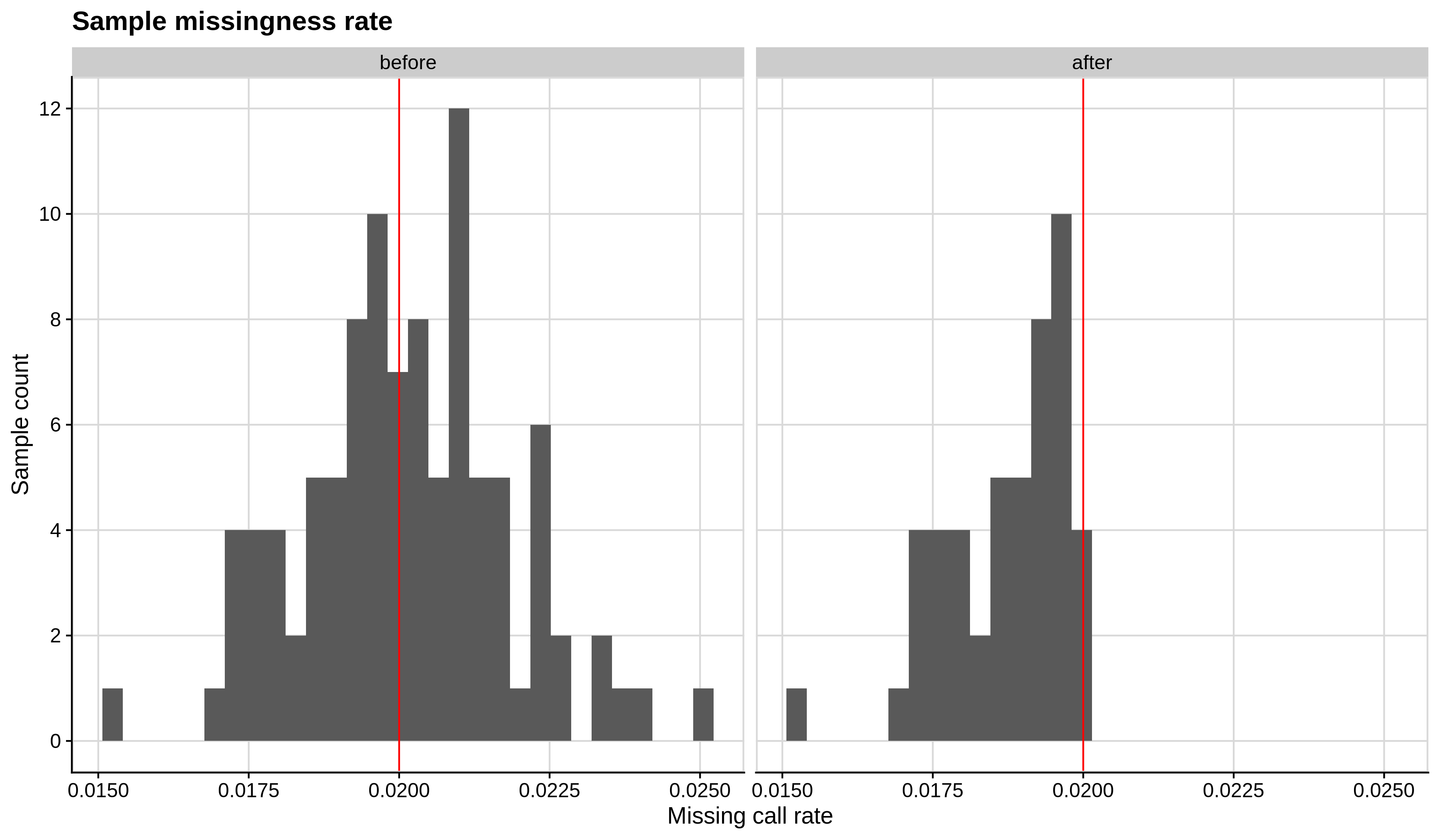
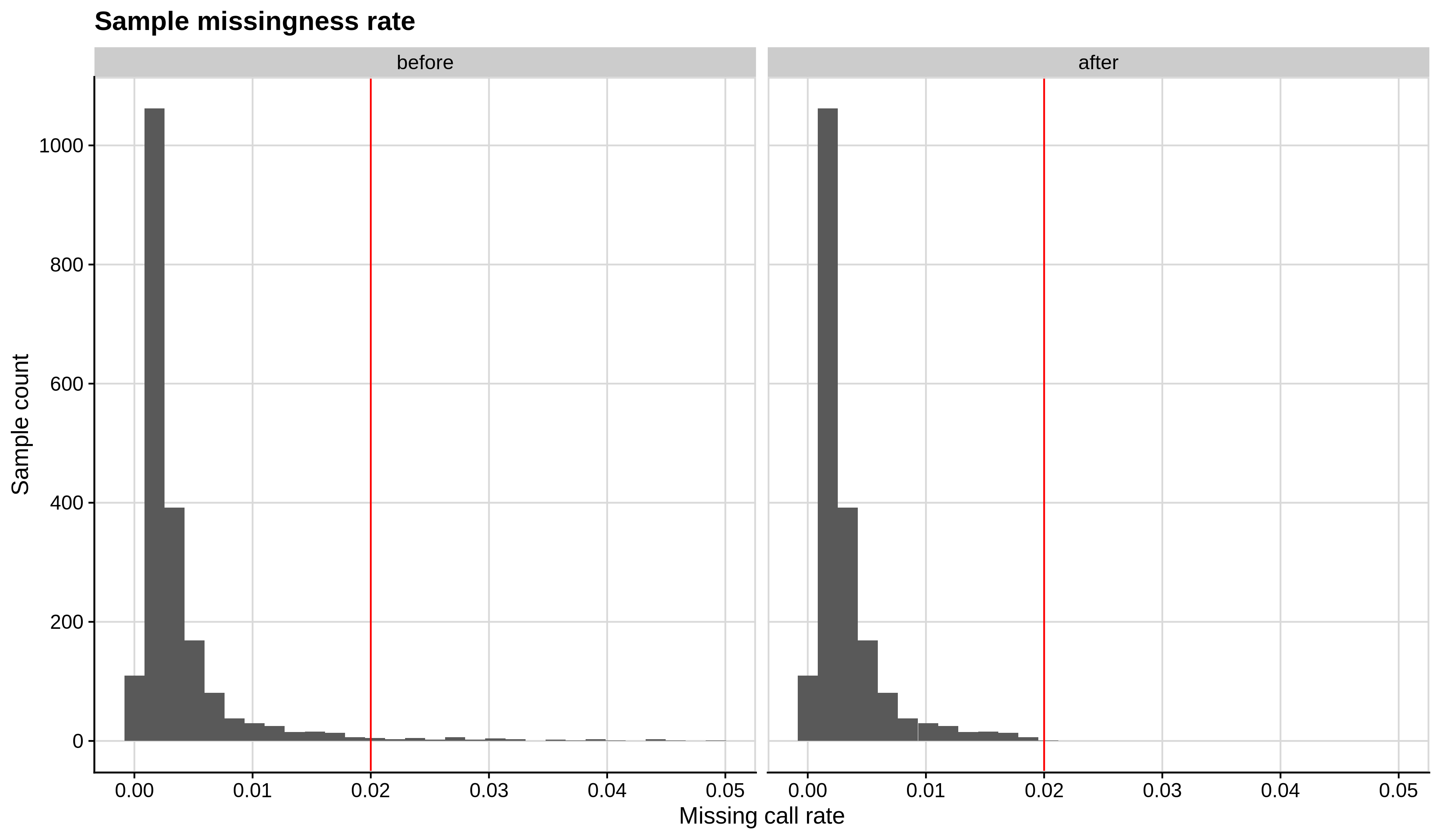
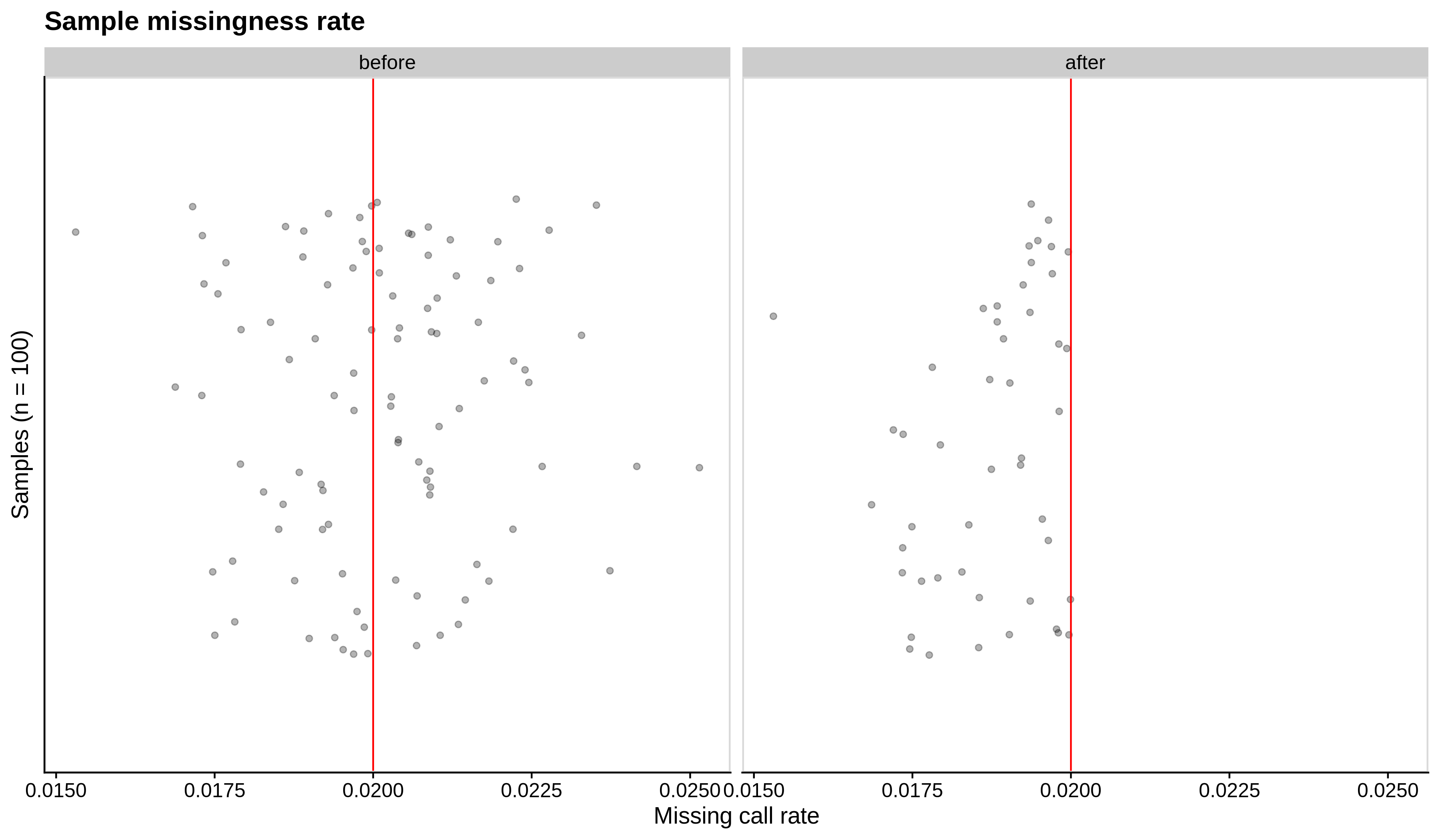
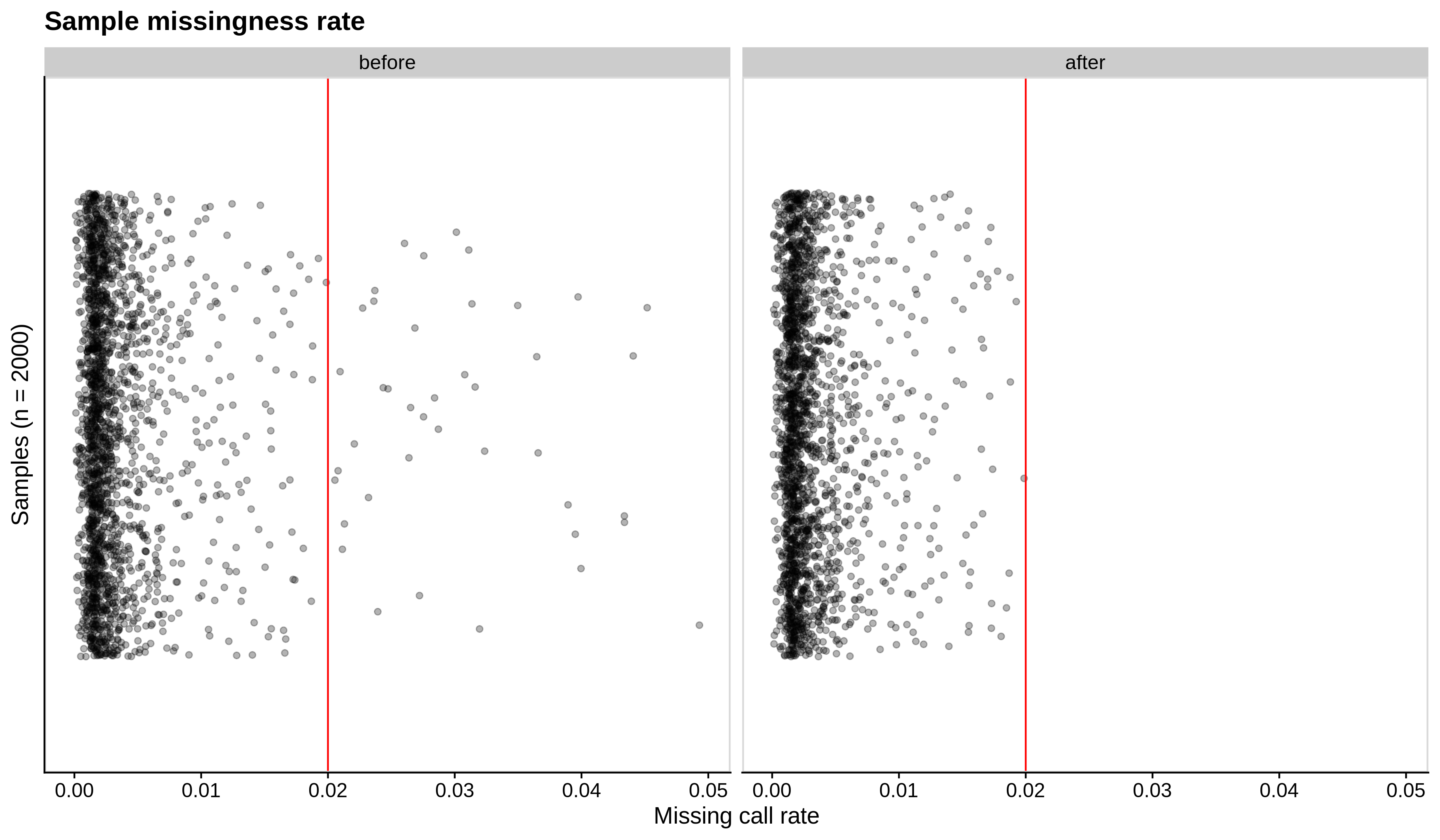
Below you can see the histograms and the scatterplots showing each metric before and after the default threshold (red line) for the toy dataset and the ALS dataset:
- Missing sample call rate check
--mind 0.02:
| Toy dataset | ALS dataset |
|---|---|
 |
 |
| Toy dataset | ALS dataset |
|---|---|
 |
 |
- Check for sex discrepancies:
| ALS dataset: All | All |
|---|---|
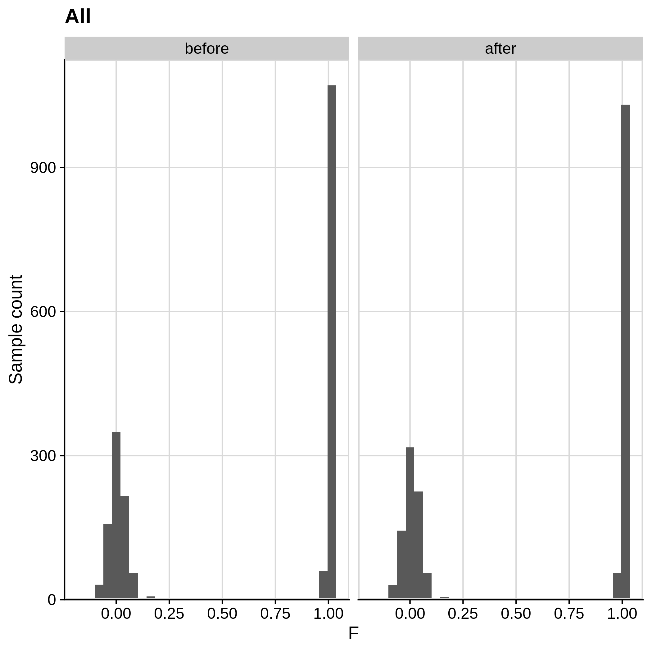 |
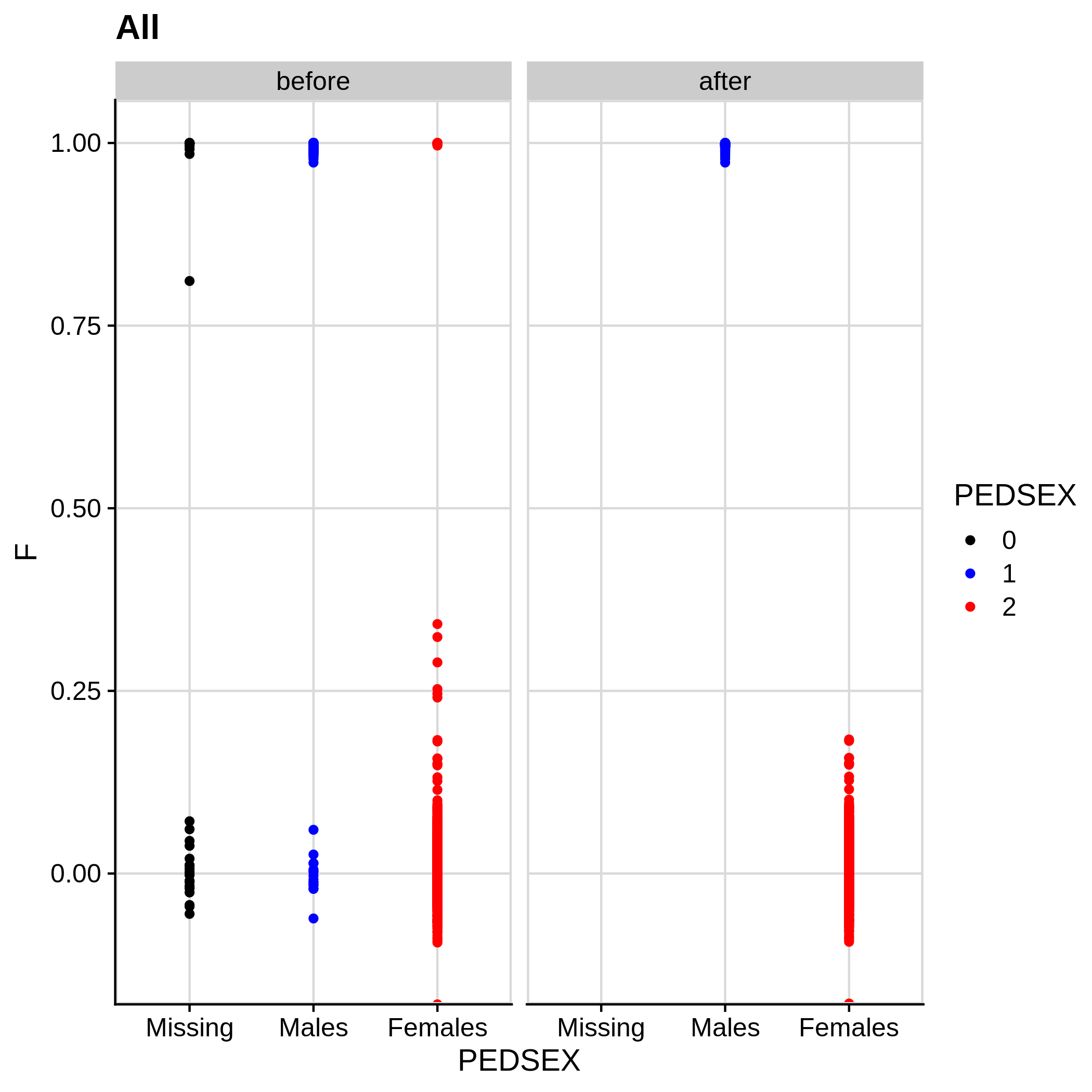 |
| ALS dataset: Women | Men |
|---|---|
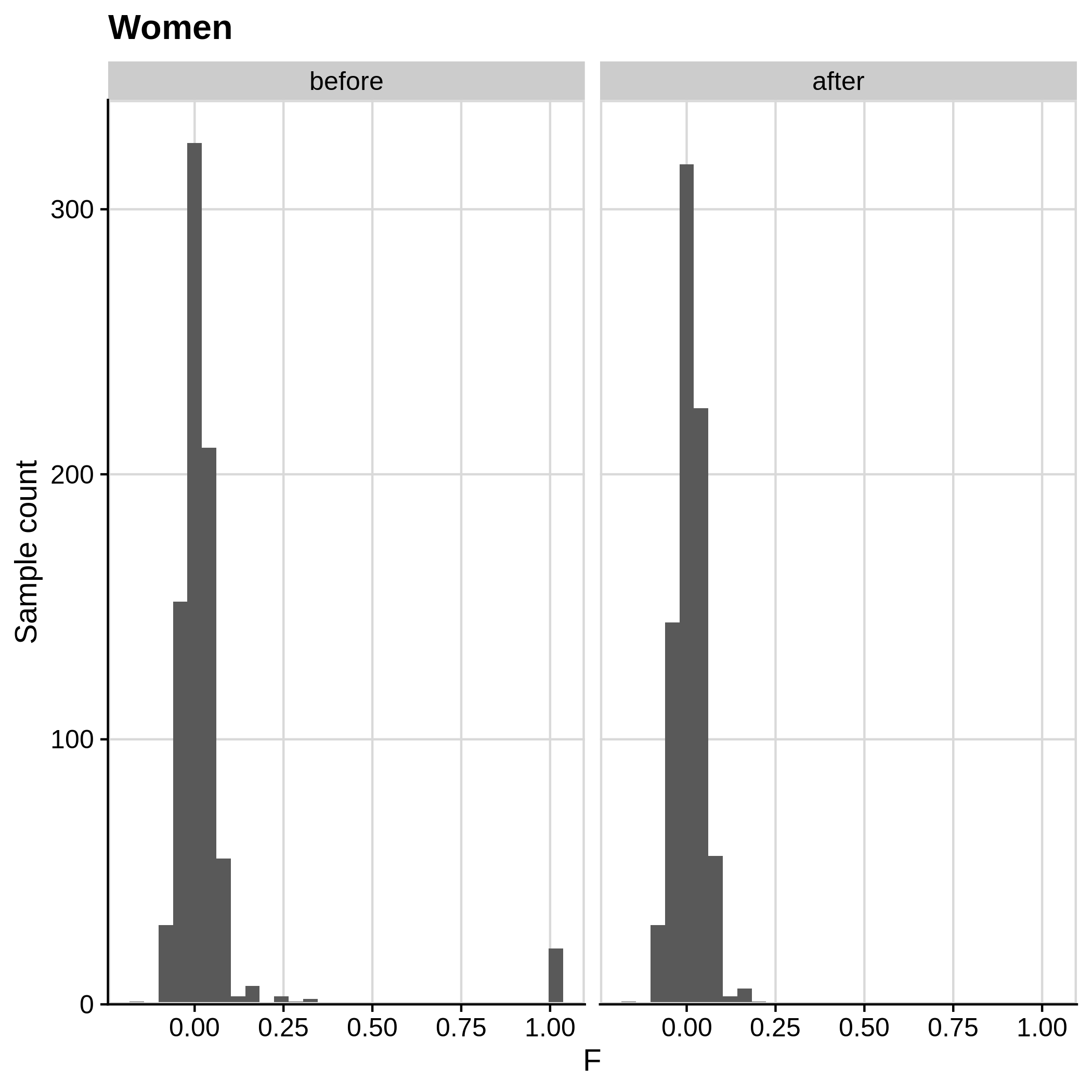 |
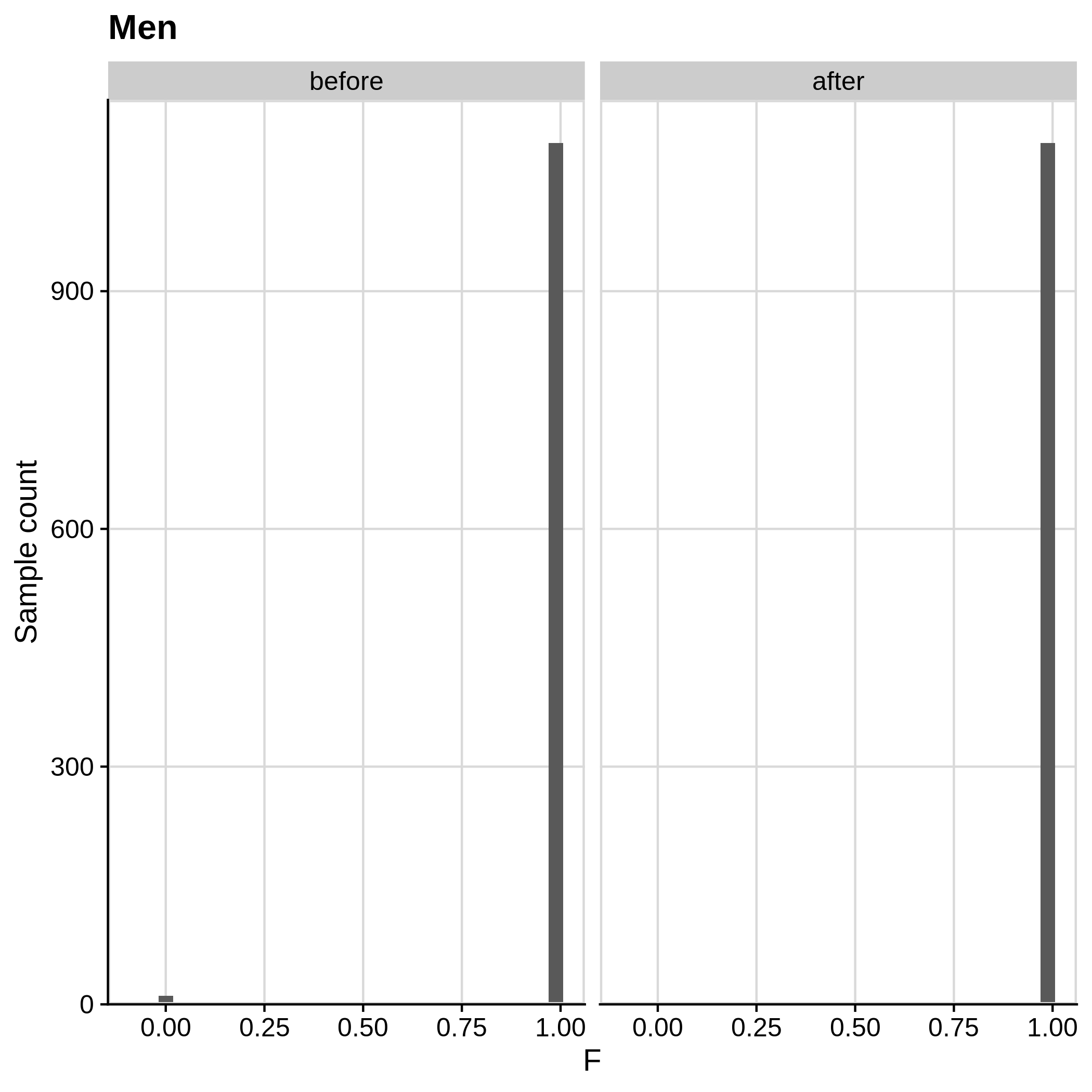 |
Note
Remember that the toy dataset does not contain any sex chromosomes, so --check-sex (through plink) can't be carried out.
- Heterozygosity rate (removing samples with more than 3 Standard Deviation units from the mean):
| Toy dataset | ALS dataset |
|---|---|
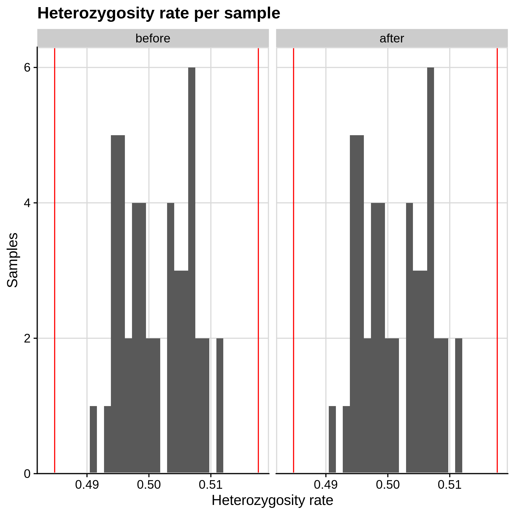 |
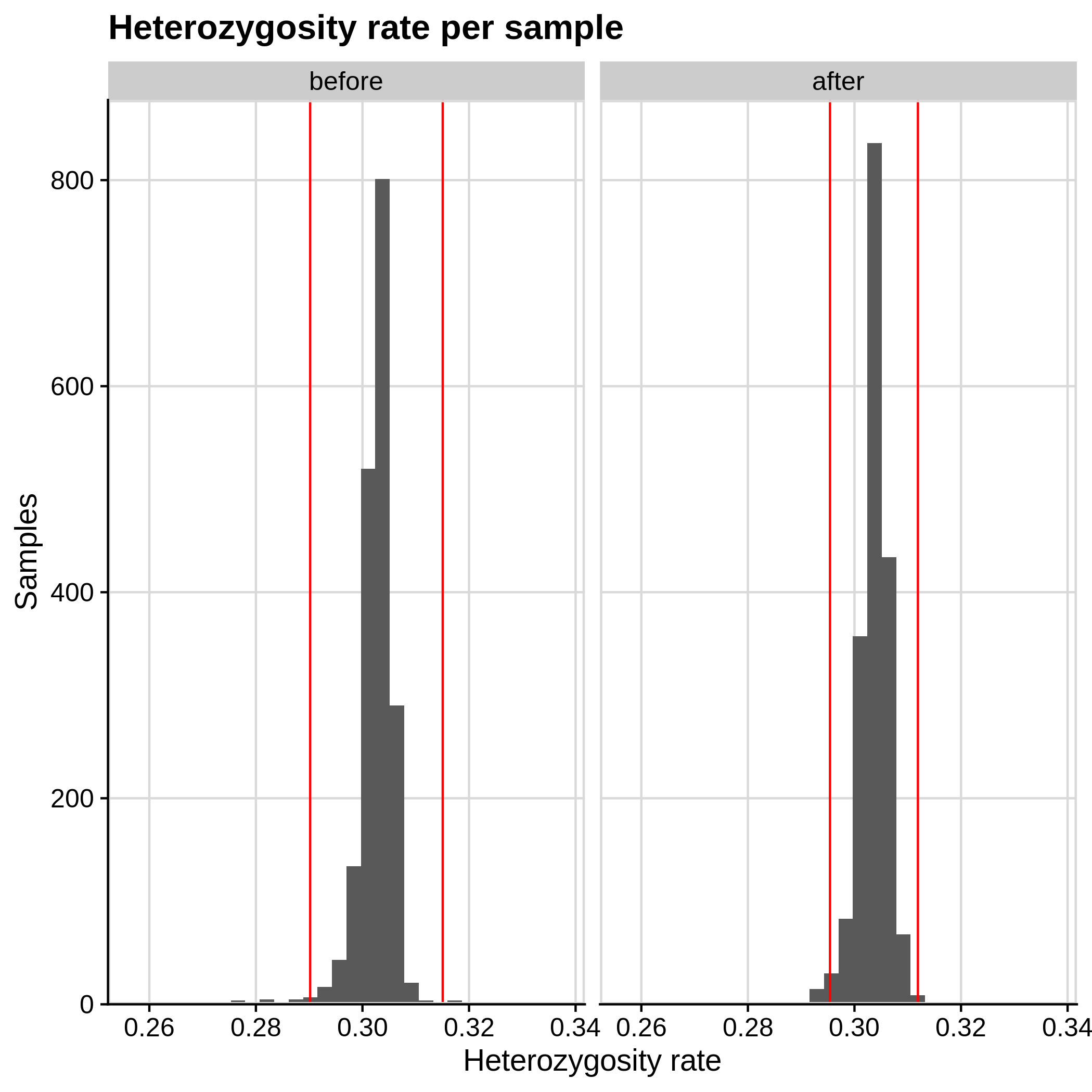 |
| Toy dataset | ALS dataset |
|---|---|
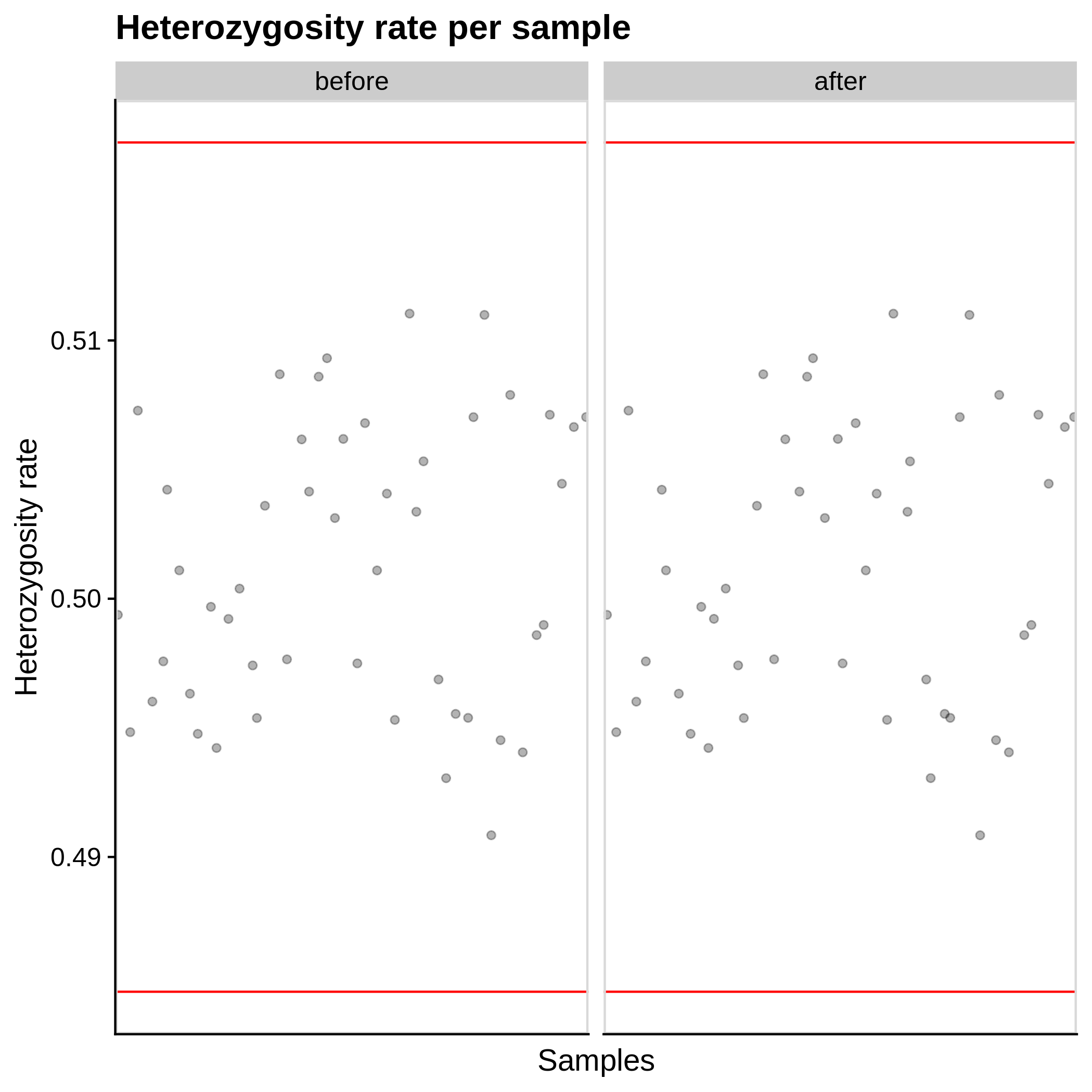 |
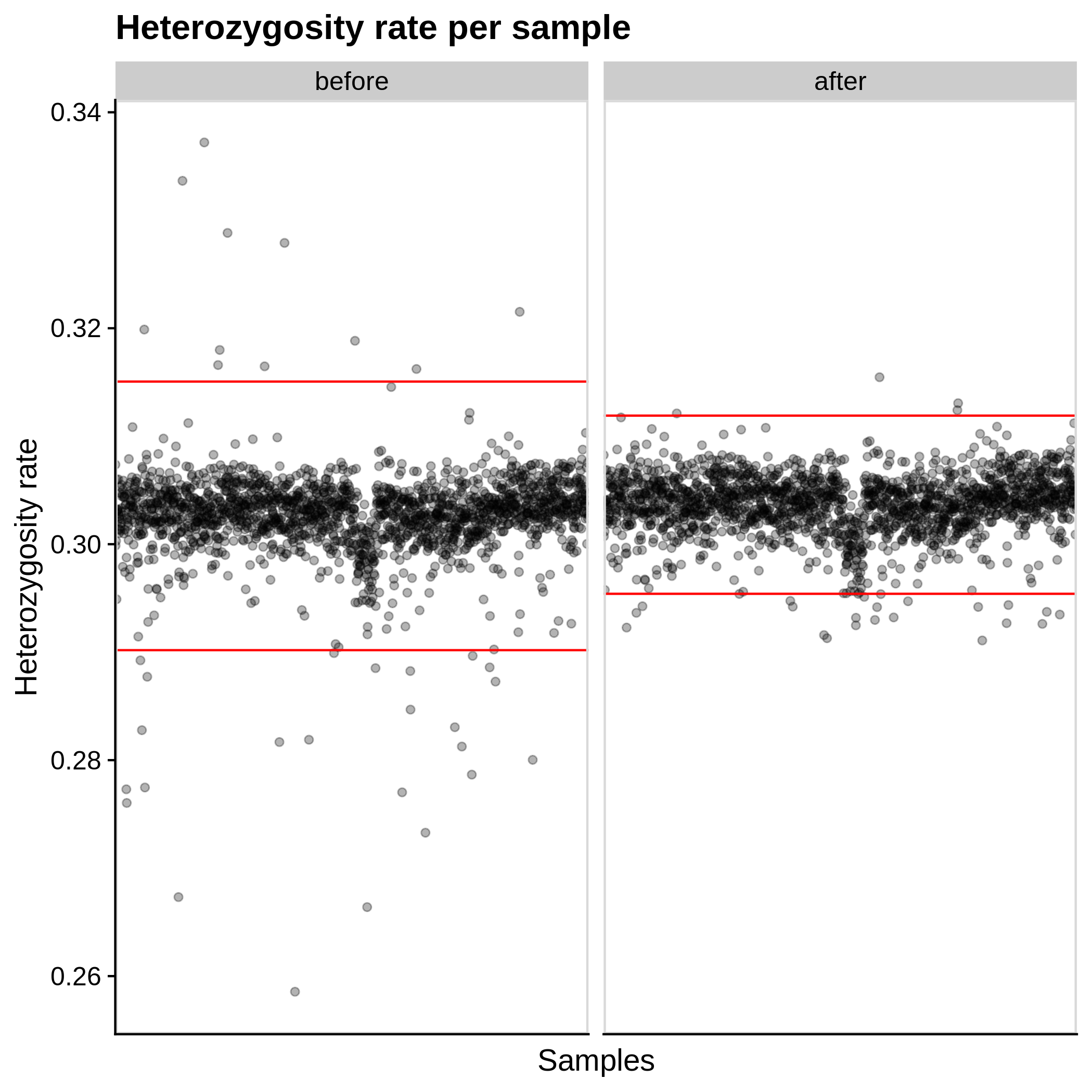 |
These are the removed samples and variants for the toy and the ALS datasets through all the steps of the sample QC:
| Toy removed samples log in sample QC | Toy removed variants log in sample QC |
|---|---|
 |
 |
| ALS removed samples log in sample QC | ALS removed variants log in sample QC |
|---|---|
 |
 |
It is normal to expect a drop in the number of variants between C1 and C2 steps, as poor quality variants are removed in B1 (--geno 0.1) and if --keep-sex-chroms false is used then a decrease between C4 and C5 is expected, as in B4 sex chromosomes are excluded. Accordingly, in the same steps of the sample log plot you observe a flat line.
Note
To remember the codes for each step visit the Workflow Descriptions section.
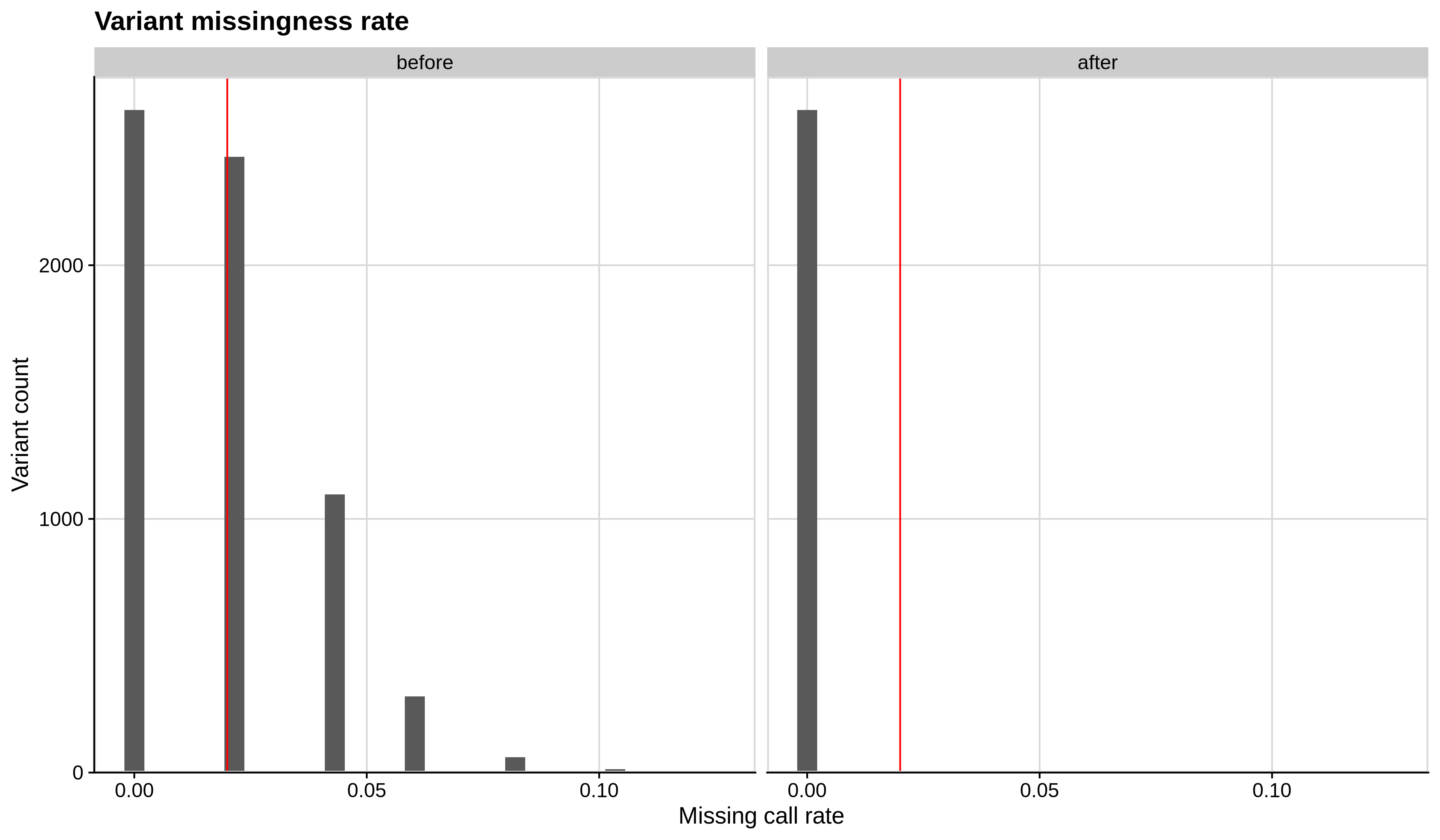
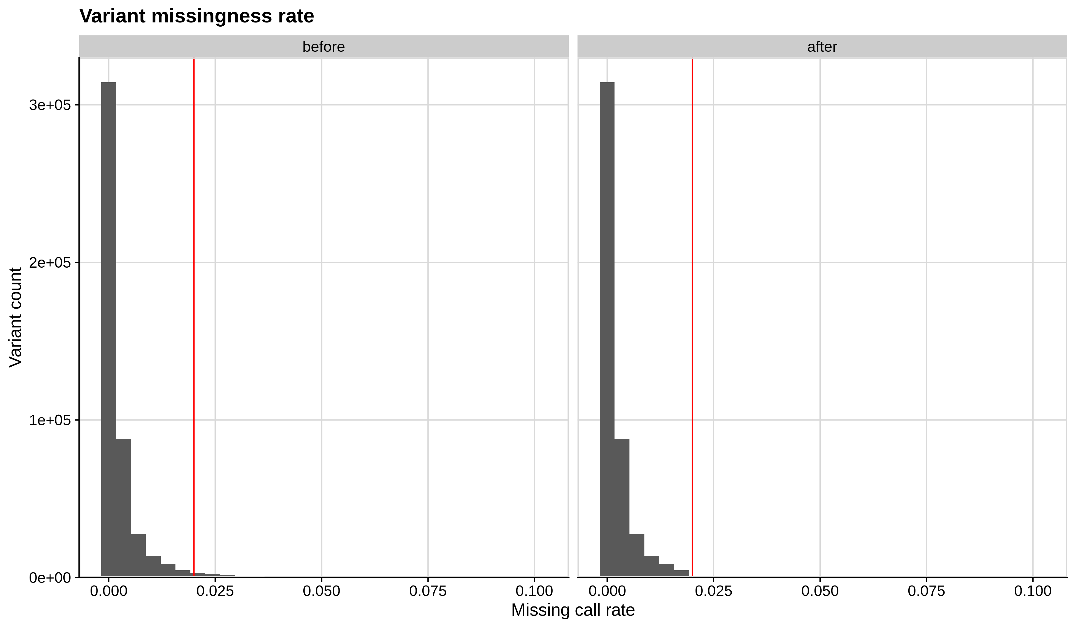
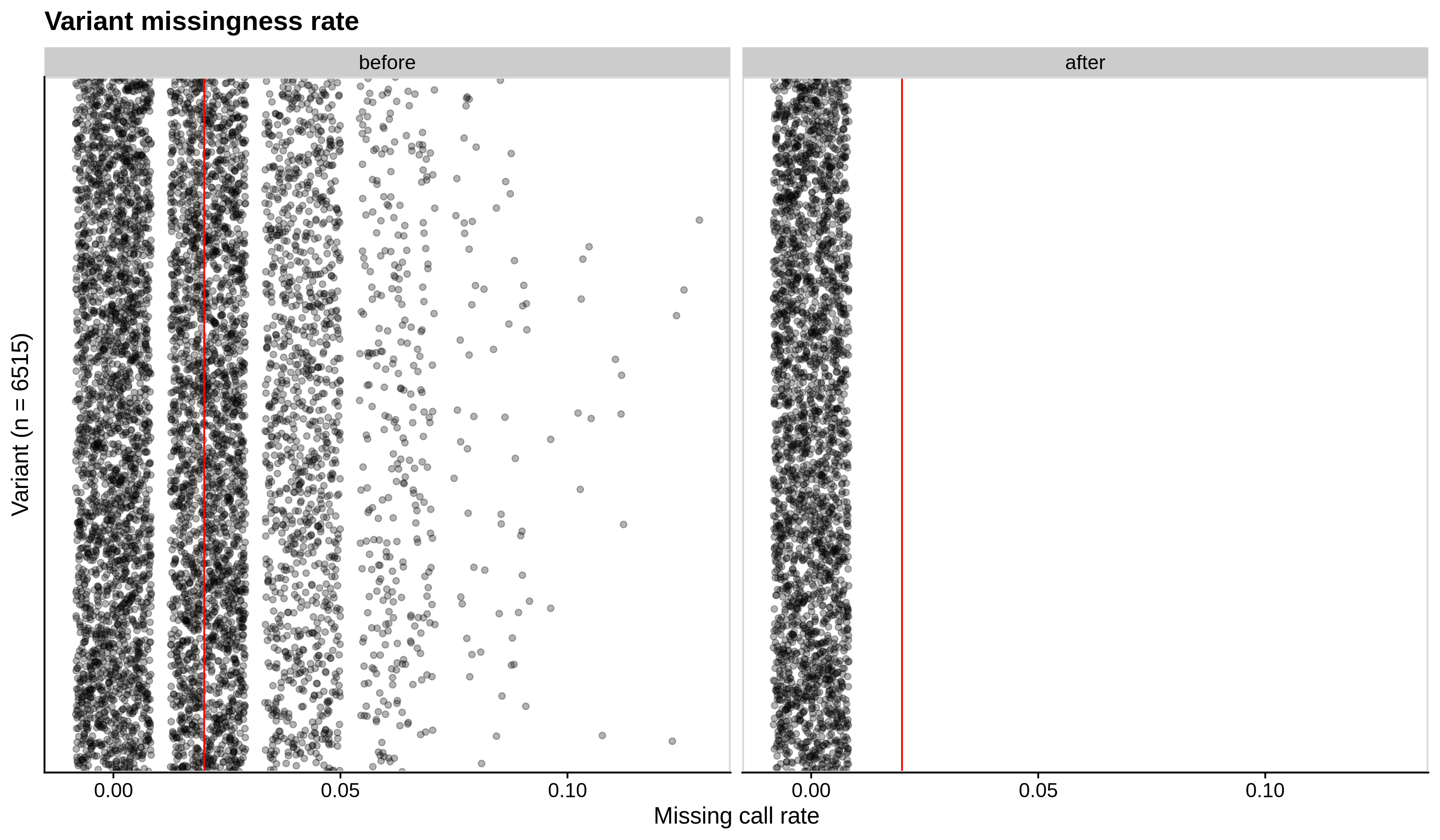
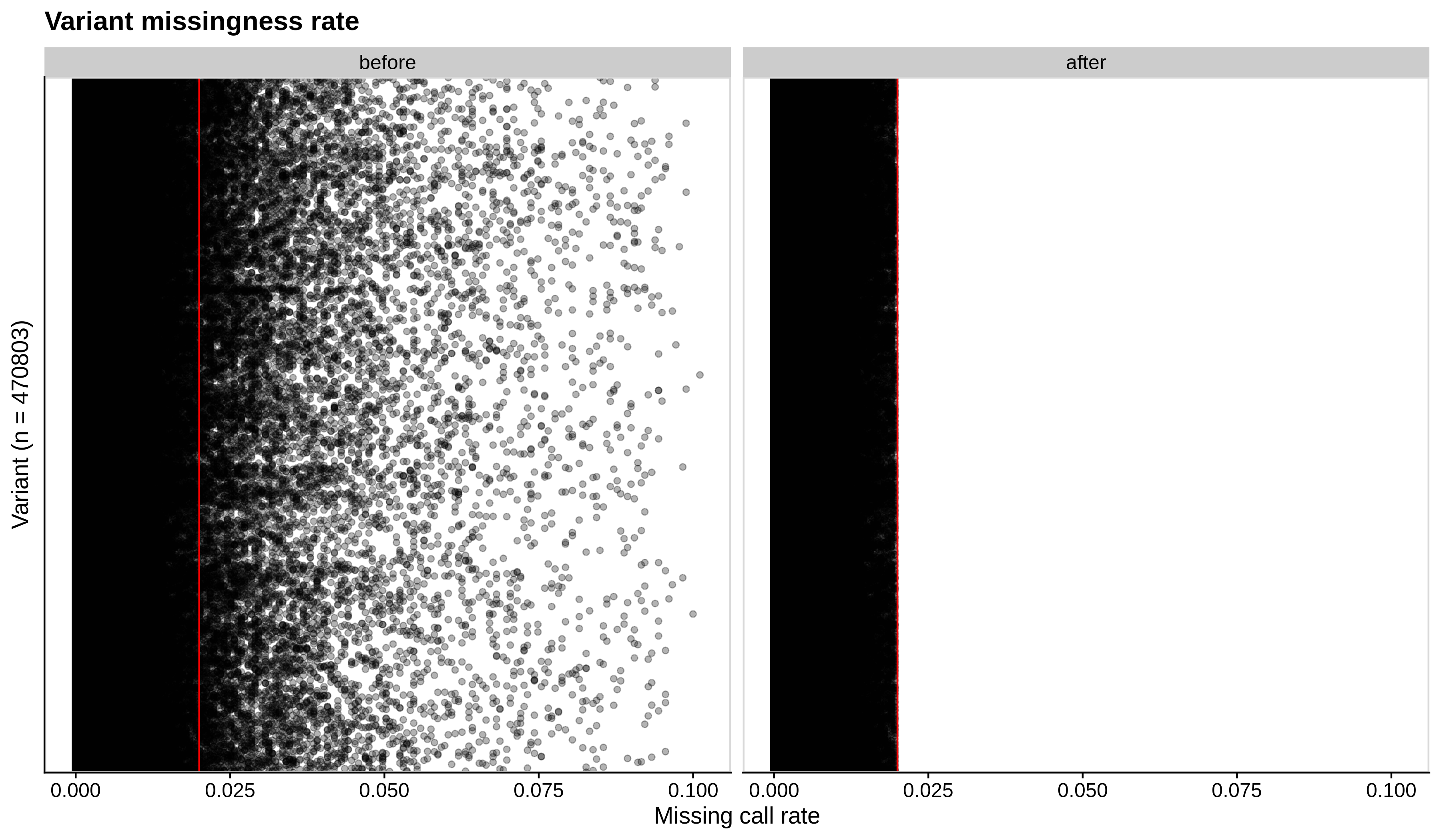
2. Variant Quality Control
Below you can see the histograms and the scatterplots showing each metric before and after the default threshold (red line) for the toy dataset and the ALS dataset:
- Missing variant call rate check
--geno 0.02:
| Toy dataset | ALS dataset |
|---|---|
 |
 |
| Toy dataset | ALS dataset |
|---|---|
 |
 |
- Hardy-Weinberg equilibrium (HWE) deviation check
--hwe 1e-7:
| Toy dataset | ALS dataset |
|---|---|
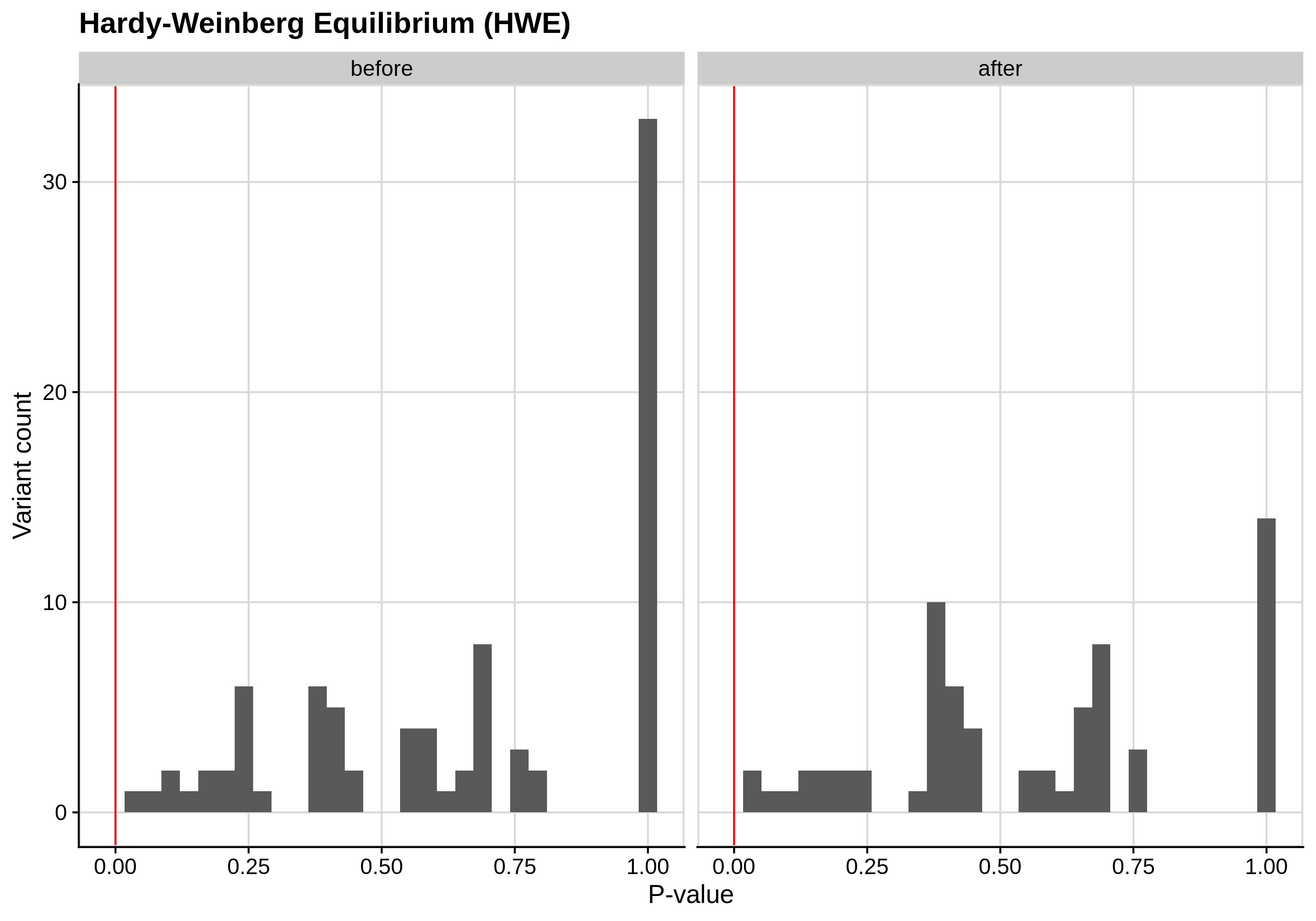 |
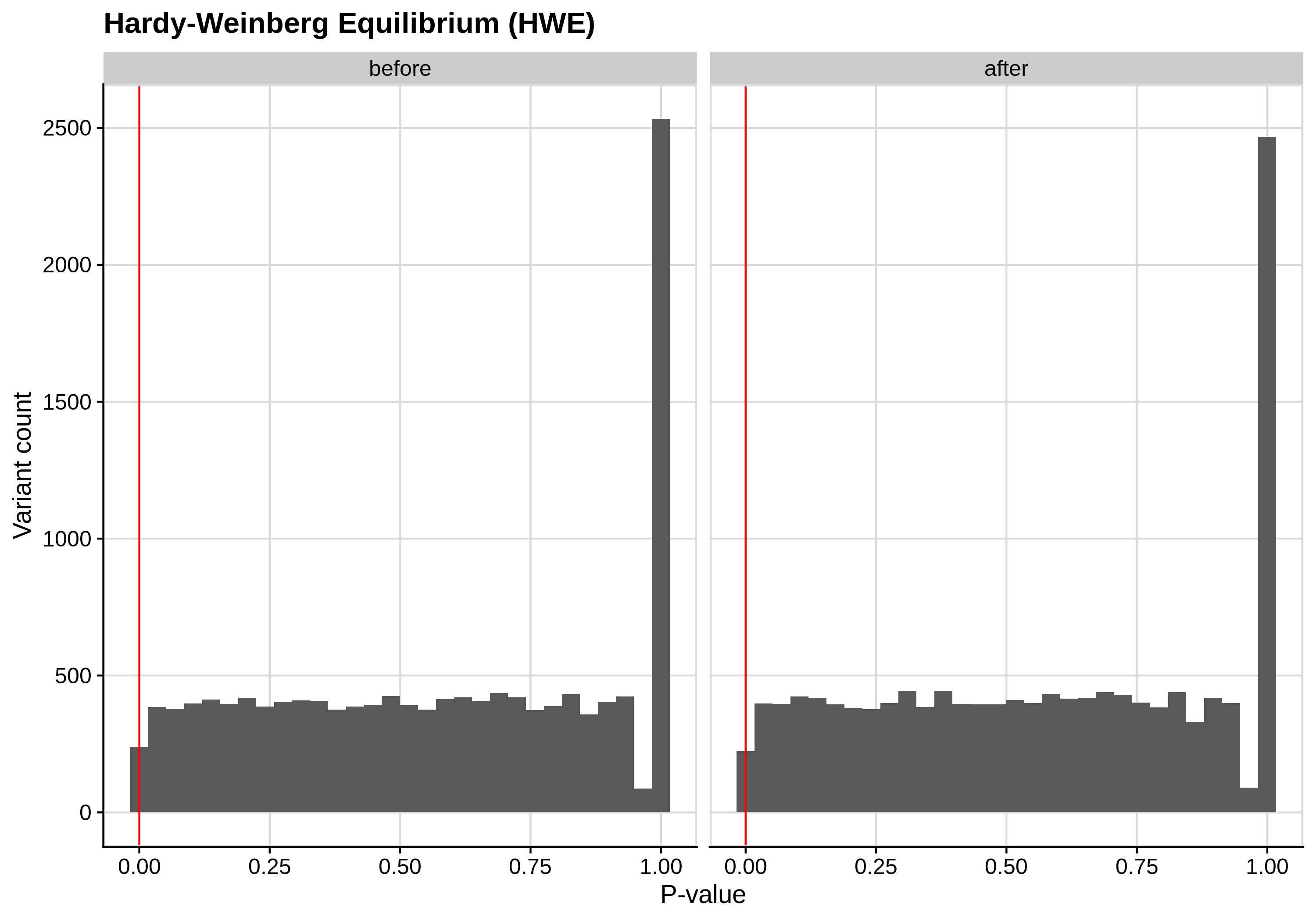 |
| Toy dataset zoomed | ALS dataset zoomed |
|---|---|
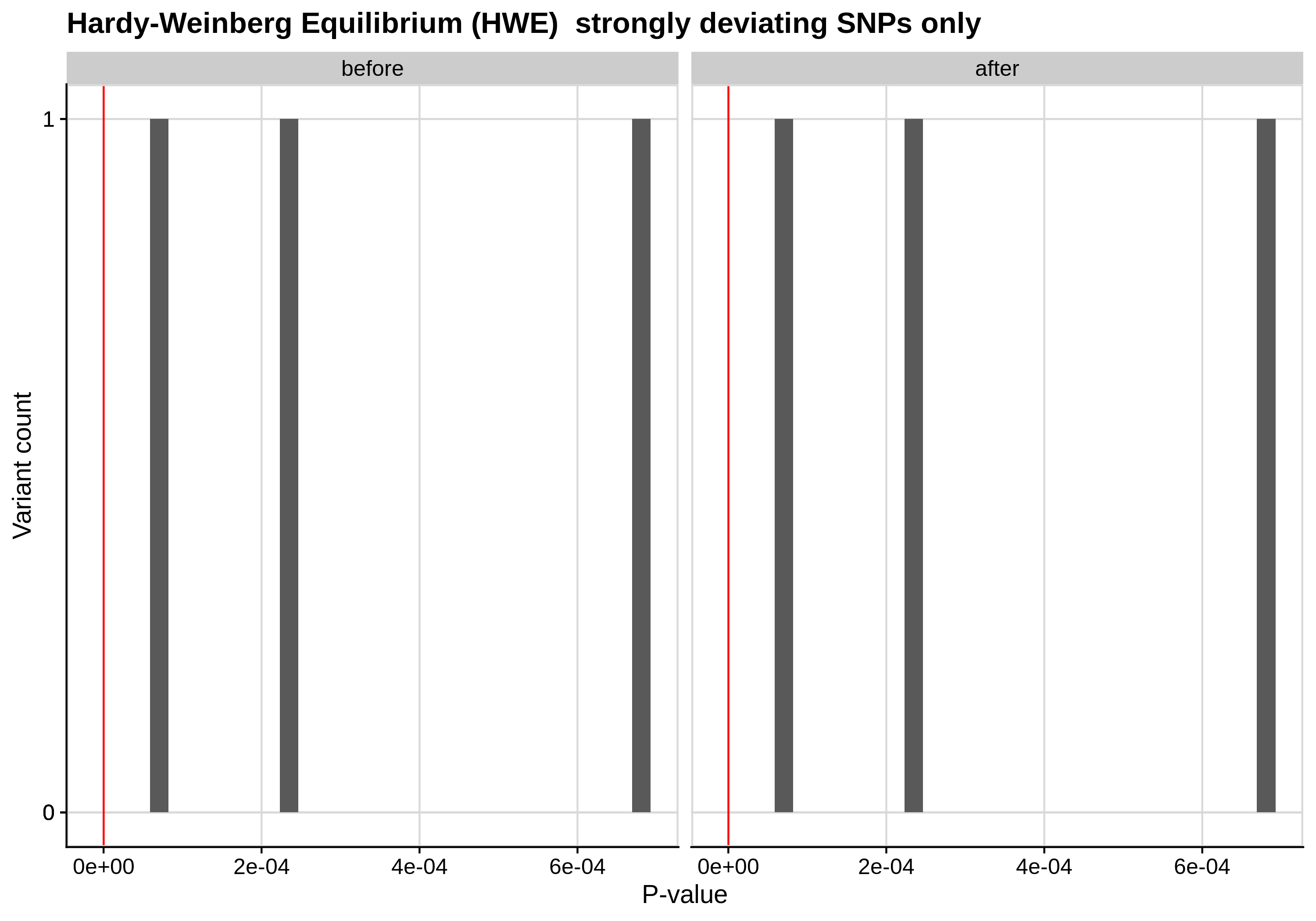 |
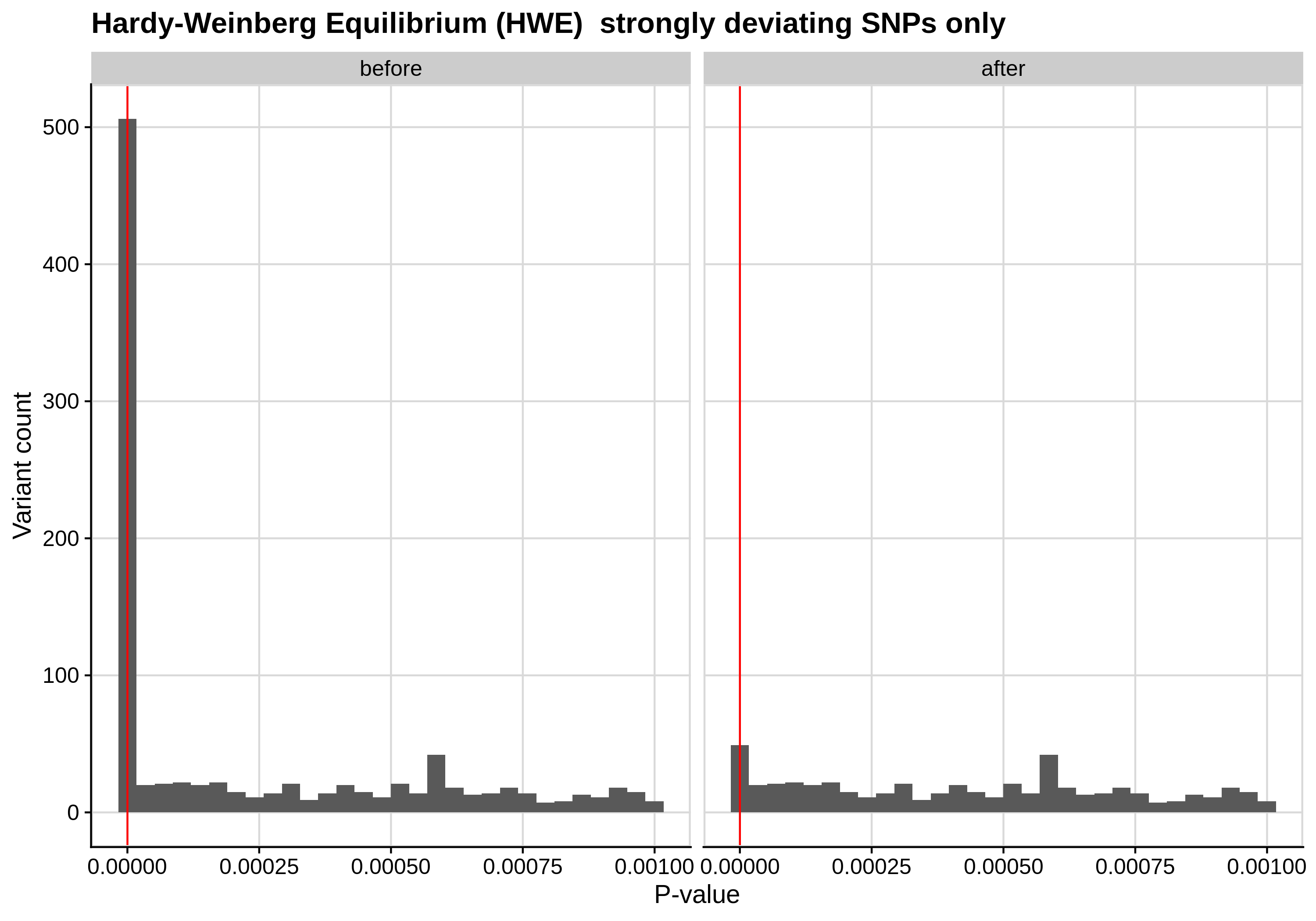 |
Since the preferred threshold is usually very low and concerns only a small fraction of the cohort, we generate two kinds of plots, one showing the distribution for the entire cohort and another one showing the distribution for samples with lower p-values (i.e. <1e-3).
- Minor Allele Frequency (MAF) check
--maf 0.05:
| Toy dataset | ALS dataset |
|---|---|
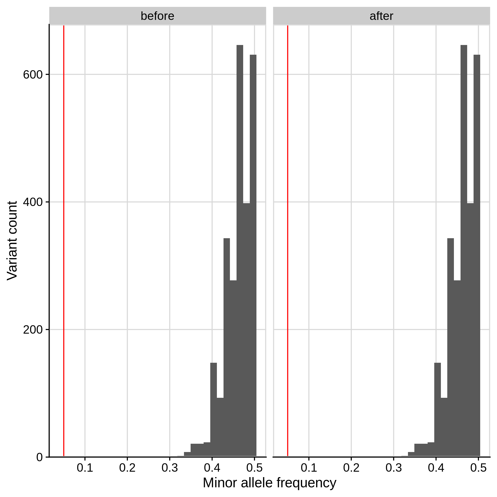 |
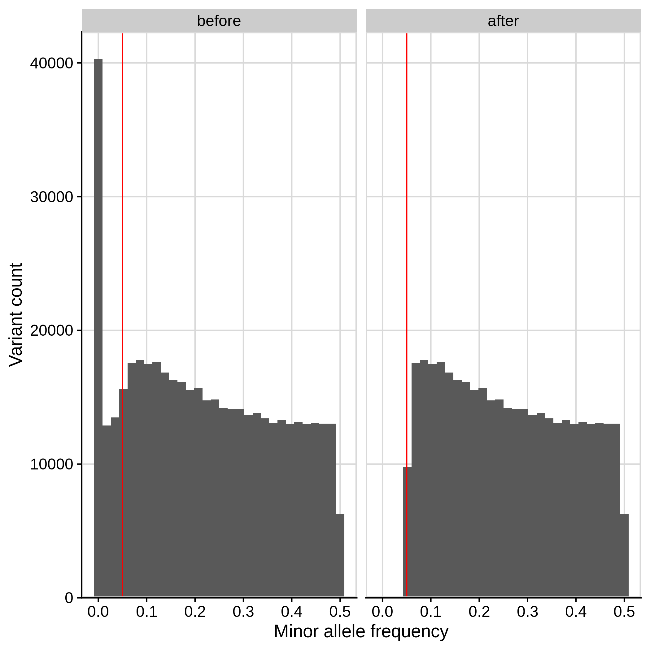 |
- Missingness in case/ control status check
--excludevariants with p-value less than 1e-7:
| Toy dataset | ALS dataset |
|---|---|
|
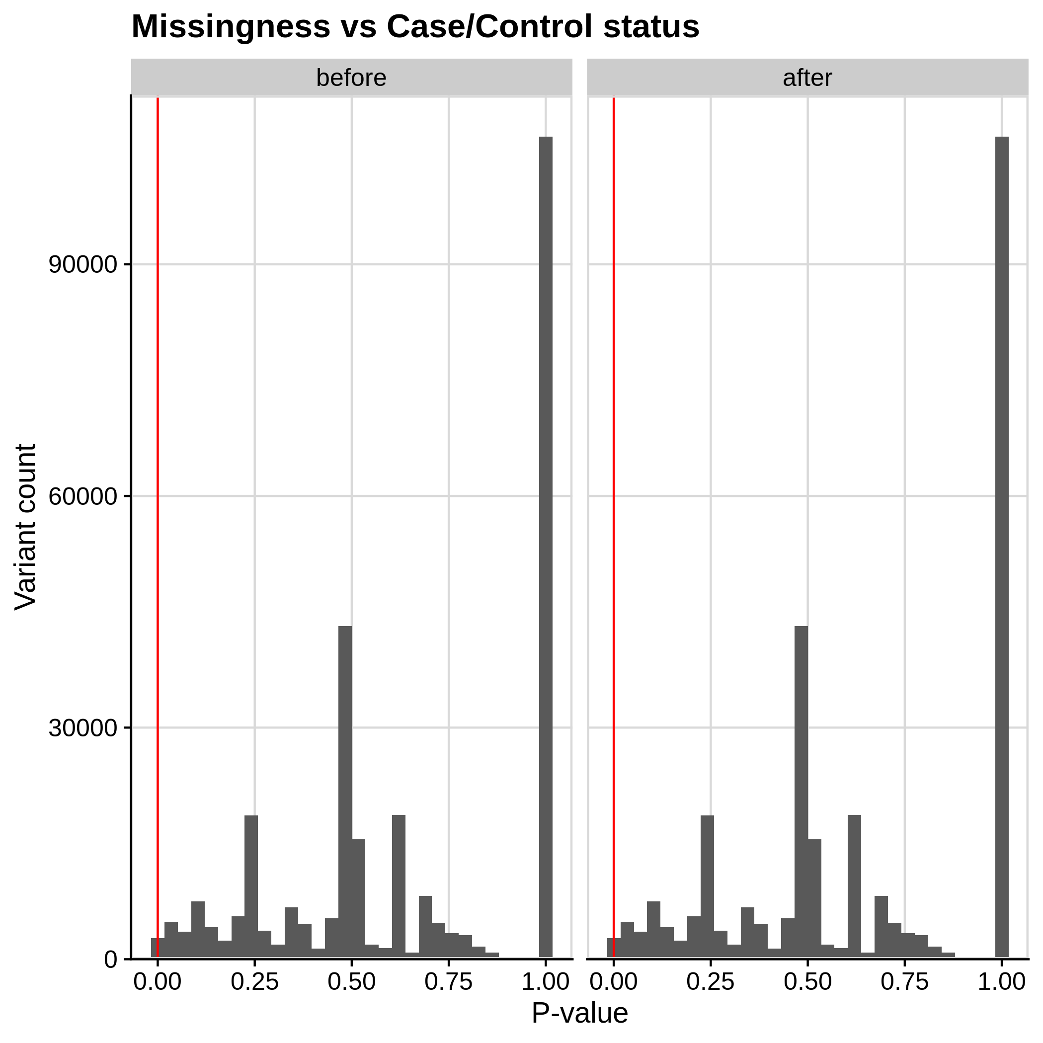 |
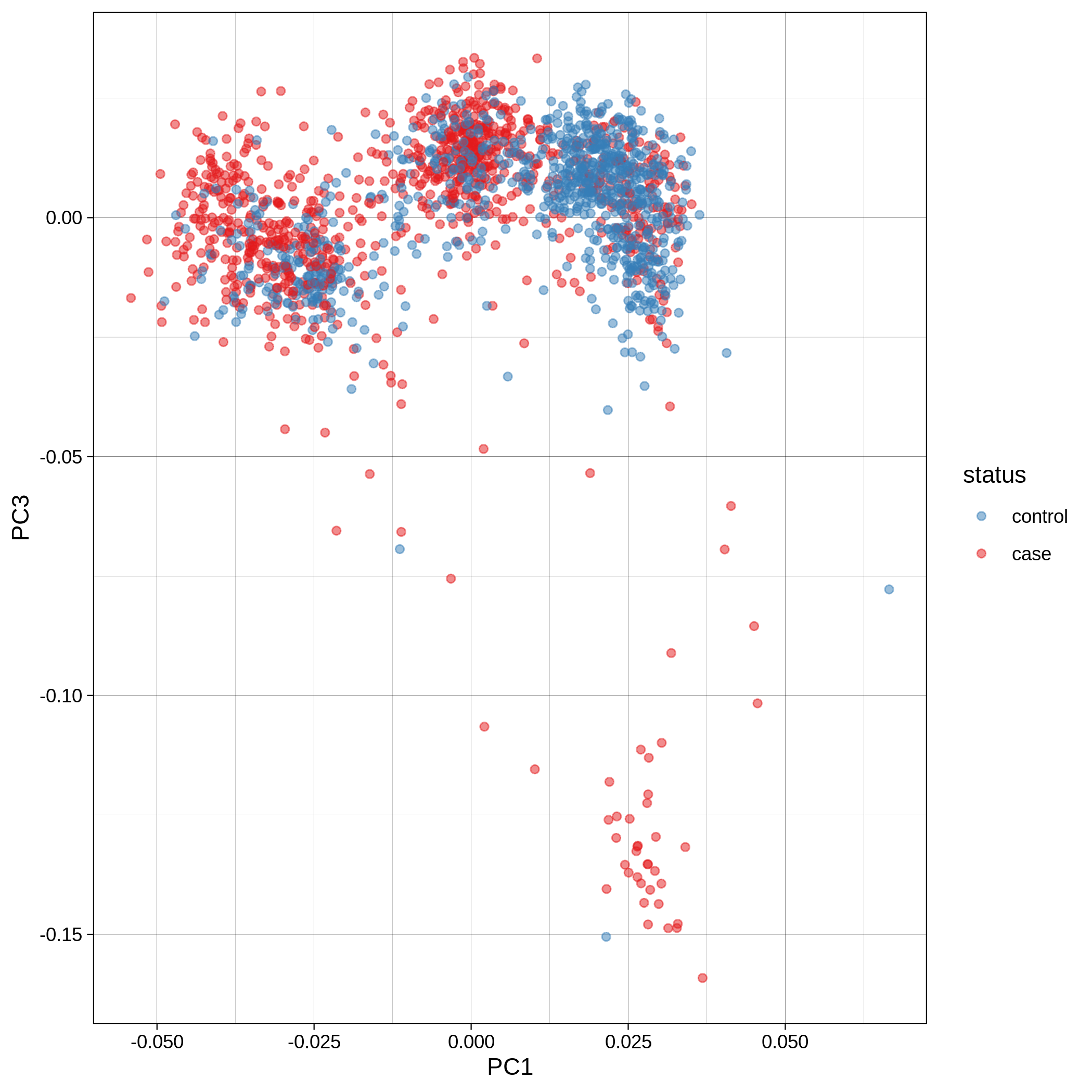
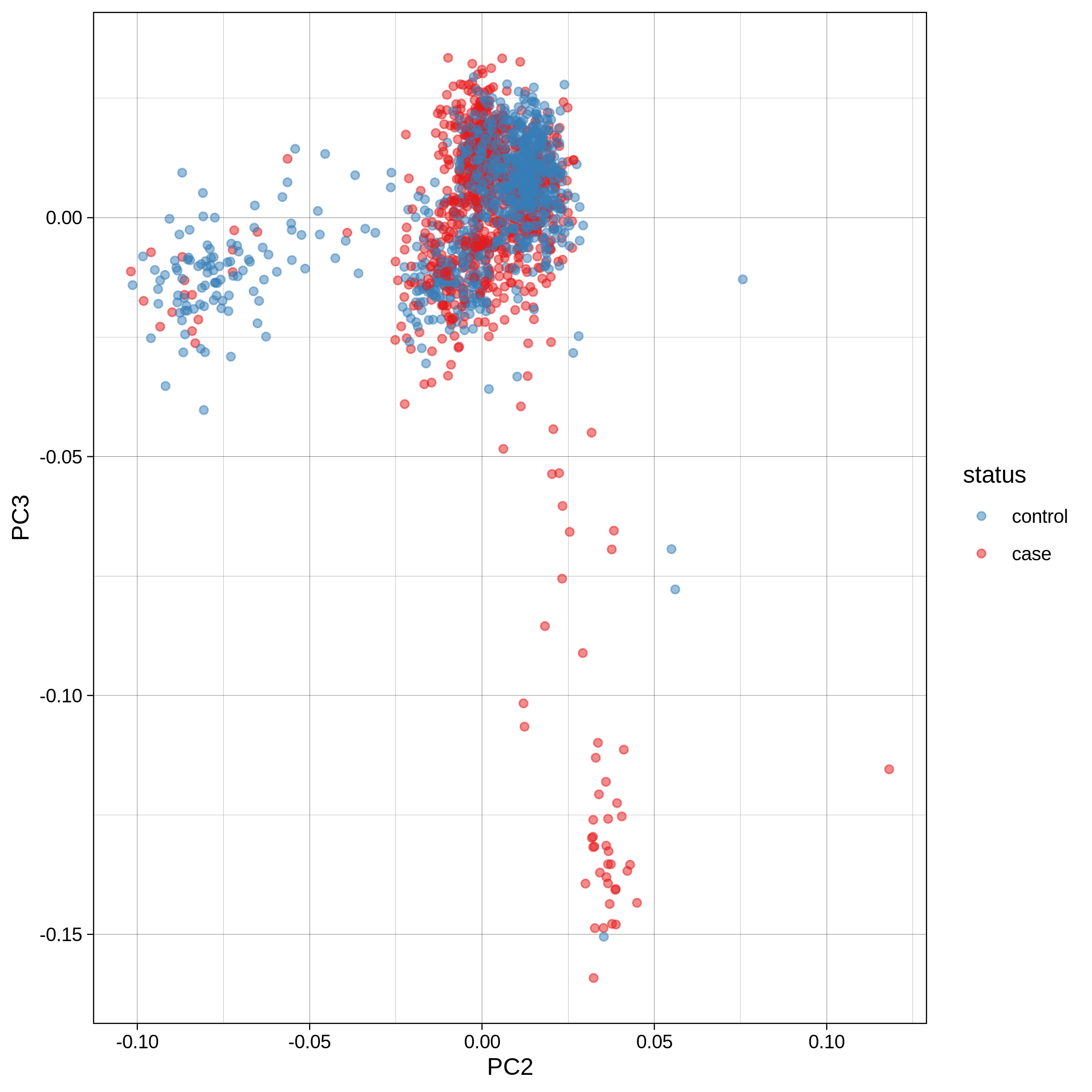
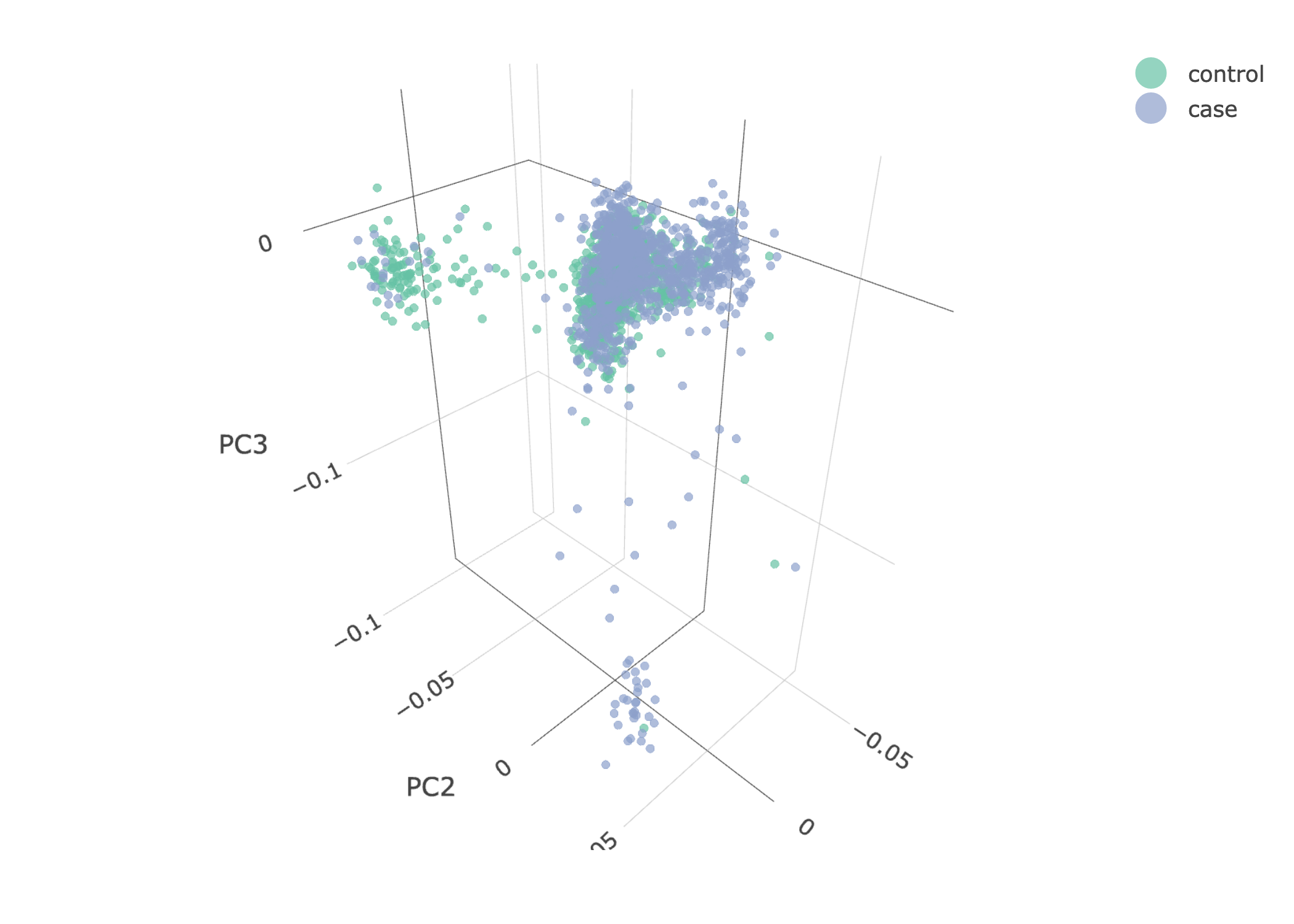
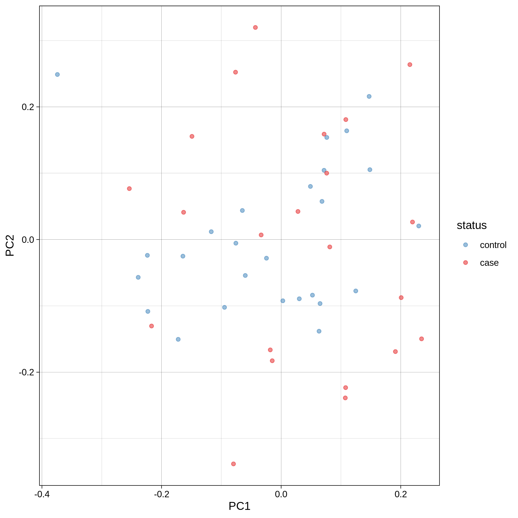
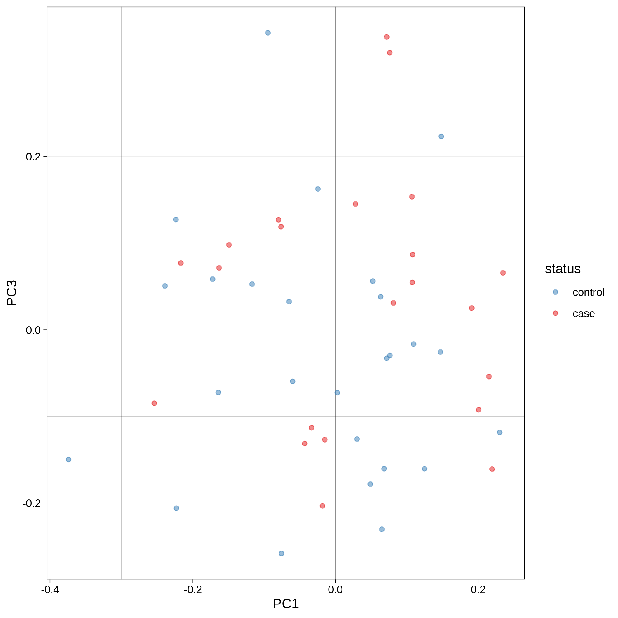
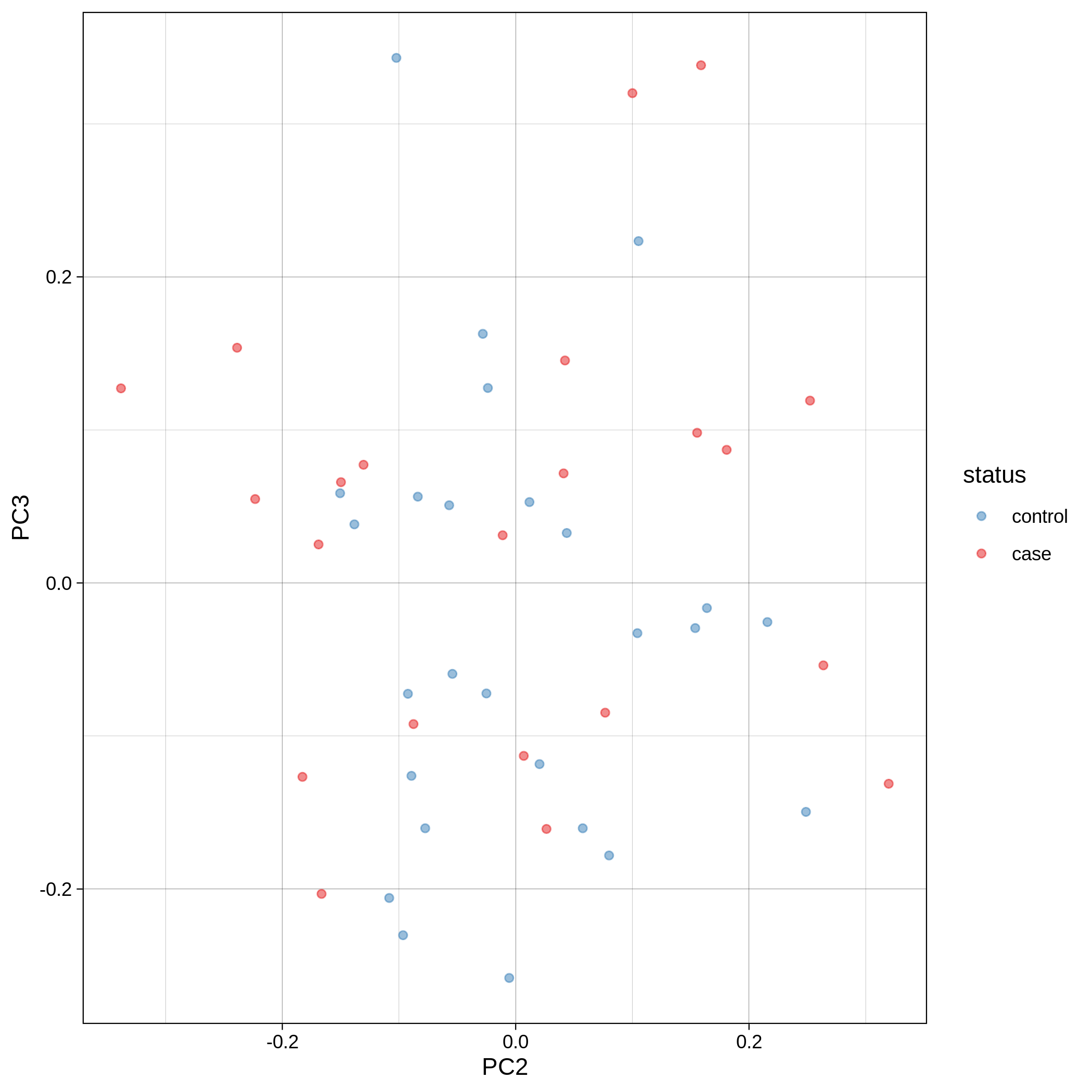
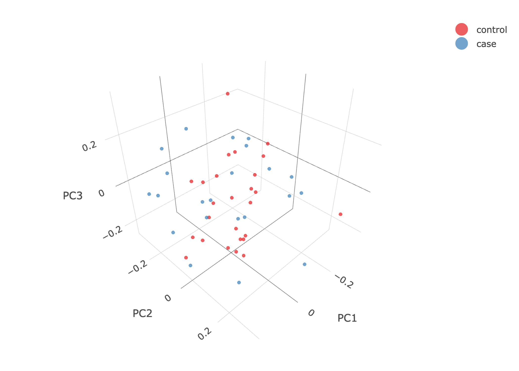
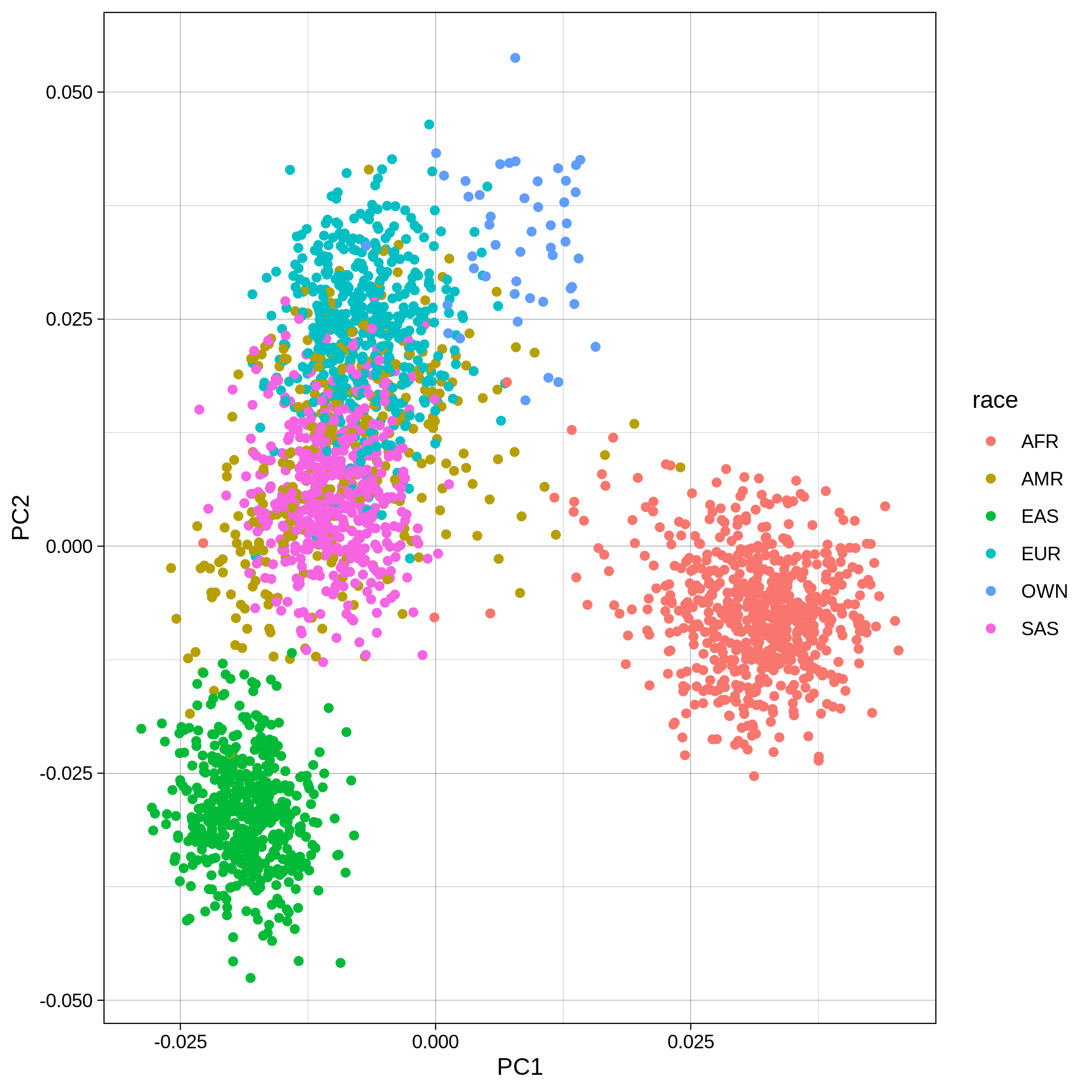
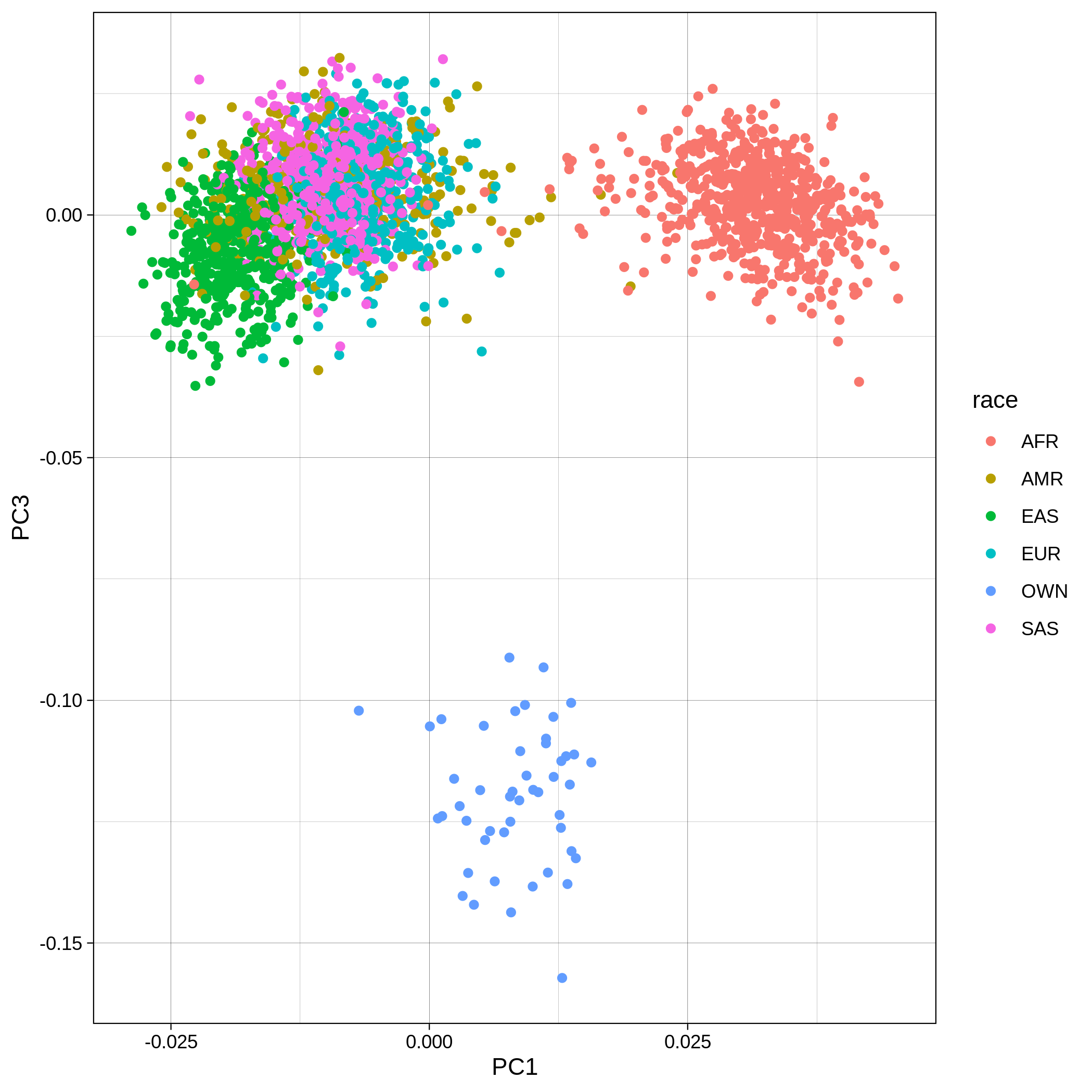
- PCA plots using only the user's data, along with case/control labels:
| ALS dataset: PC1vsPC2 | ALS dataset: PC1vsPC3 |
|---|---|
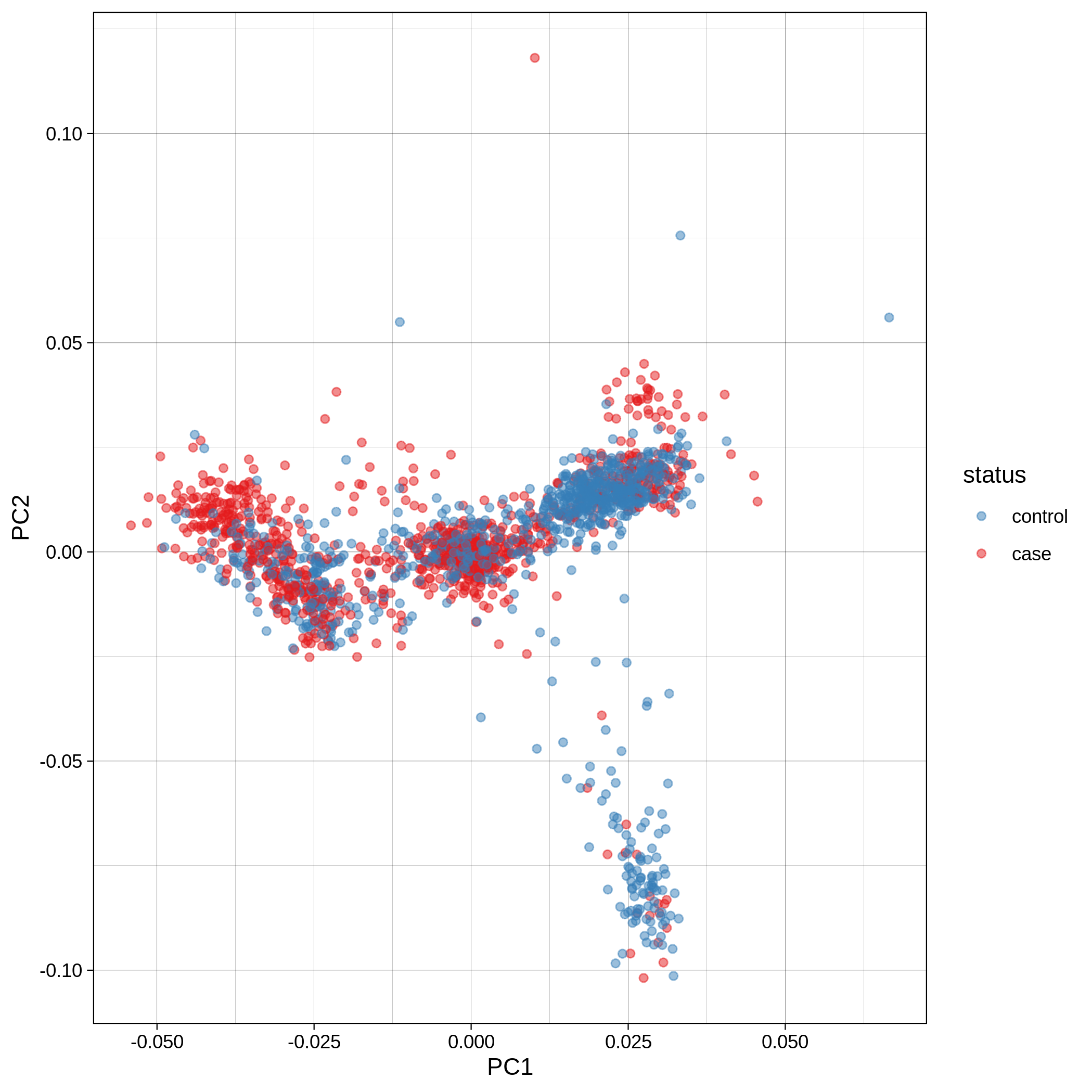 |
 |
| ALS dataset: PC2vsPC3 | ALS dataset: 3D PCA |
|---|---|
 |
 |
| Toy dataset: PC1vsPC2 | Toy dataset: PC1vsPC3 |
|---|---|
 |
 |
| Toy dataset: PC2vsPC3 | Toy dataset: 3D PCA |
|---|---|
 |
 |
Note
Since we have used --pop_strat, the Principal Component Analysis in the Variant QC workflow is run AFTER population stratification. This means that the PCA plots at this stage reflect genetically homogenous samples. If you didn't use --pop_strat then variant QC would still run, producing in the end PCA plots potentially with outliers.
These are the removed samples and variants for the toy and the ALS datasets through all the steps of the variant QC:
| Toy removed samples log in variant QC | Toy removed variants log in variant QC |
|---|---|
 |
 |
| ALS removed samples log in variant QC | ALS removed variants log in variant QC |
|---|---|
 |
 |
Note
To remember the codes for each step visit the Workflow Descriptions section.
Population Stratification --pop_strat
Within the results_toy/pop_strat/ folder you will see:
- One HTML report including the following plots
- Three folders:
logs/,figures/andbfiles/. Thebfiles/folder also contains the logistic analysis results with and without covariates.
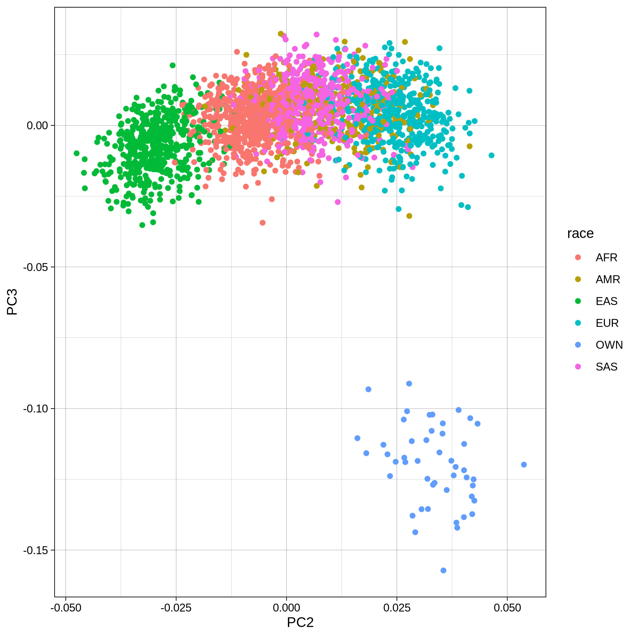
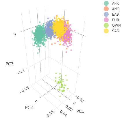
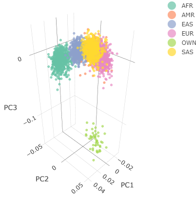
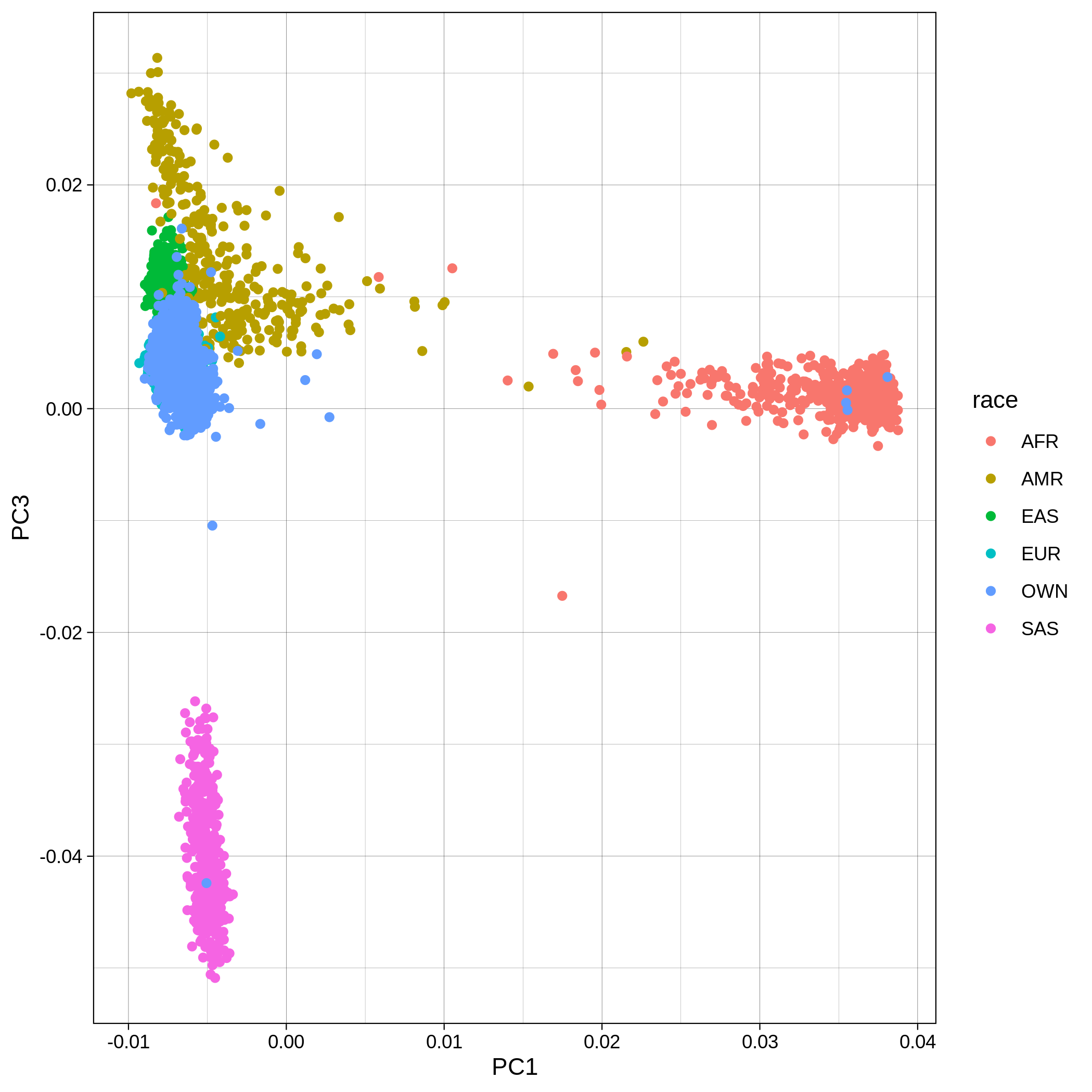
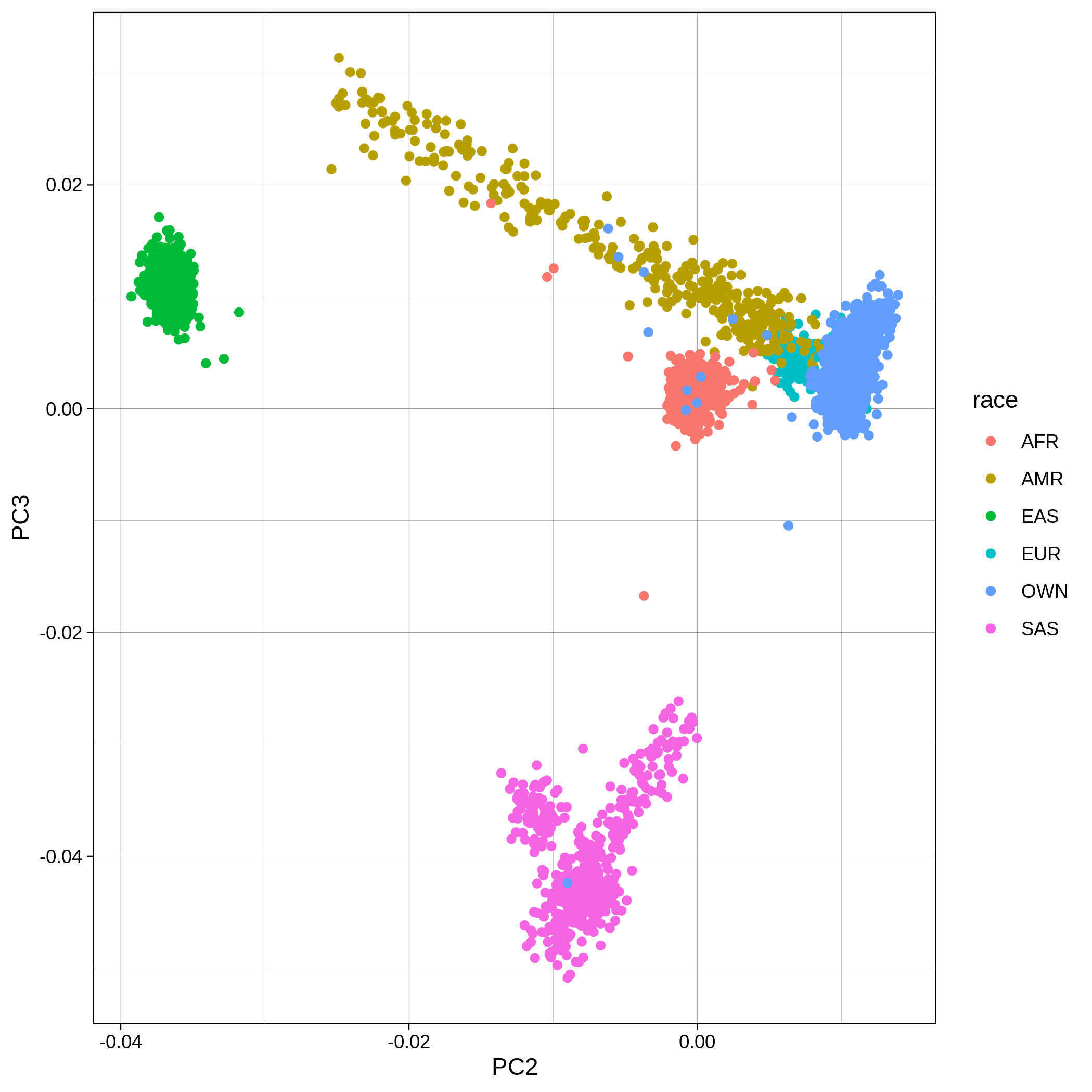
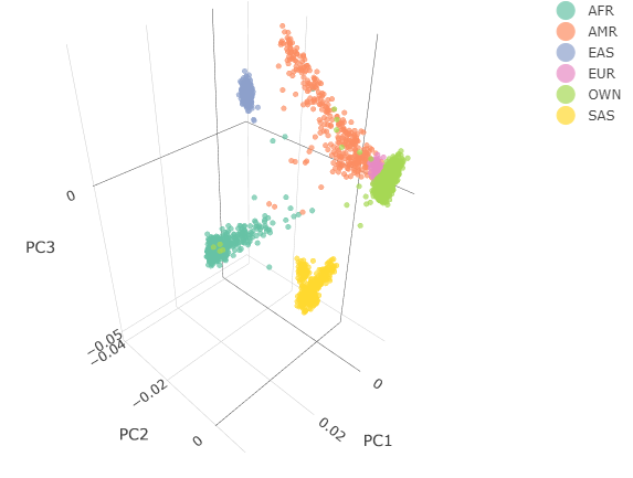
Below you can see the 2D and 3D Principal Component Analysis plots including user's data (labelled OWN) and 1,000 human genome populations before and after the removal of any outliers for the toy dataset and the ALS dataset:
| Toy dataset: PC1vsPC2 before removal | Toy dataset: PC1vsPC2 after removal |
|---|---|
 |
 |
| Toy dataset: PC1vsPC3 before removal | Toy dataset: PC1vsPC3 after removal |
|---|---|
 |
 |
| Toy dataset: PC2vsPC3 before removal | Toy dataset: PC2vsPC3 after removal |
|---|---|
 |
 |
| Toy dataset: 3D PCA before removal | Toy dataset: 3D PCA after removal |
|---|---|
 |
 |
Note
The PCA topology of the toy dataset is quite different from that of the ALS dataset, since the toy dataset is artificially made by plink2 as well as containing only a few thousand genotypes of chromosome 1, which are subsequently pruned, leaving a few hundred independent SNPs merged with 1,000 human genomes data. Keep in mind that your PCA should more likely resemble the topology of the merged ALS and 1,000 genome data.
| ALS dataset: PC1vsPC2 before removal | ALS dataset: PC1vsPC2 after removal |
|---|---|
 |
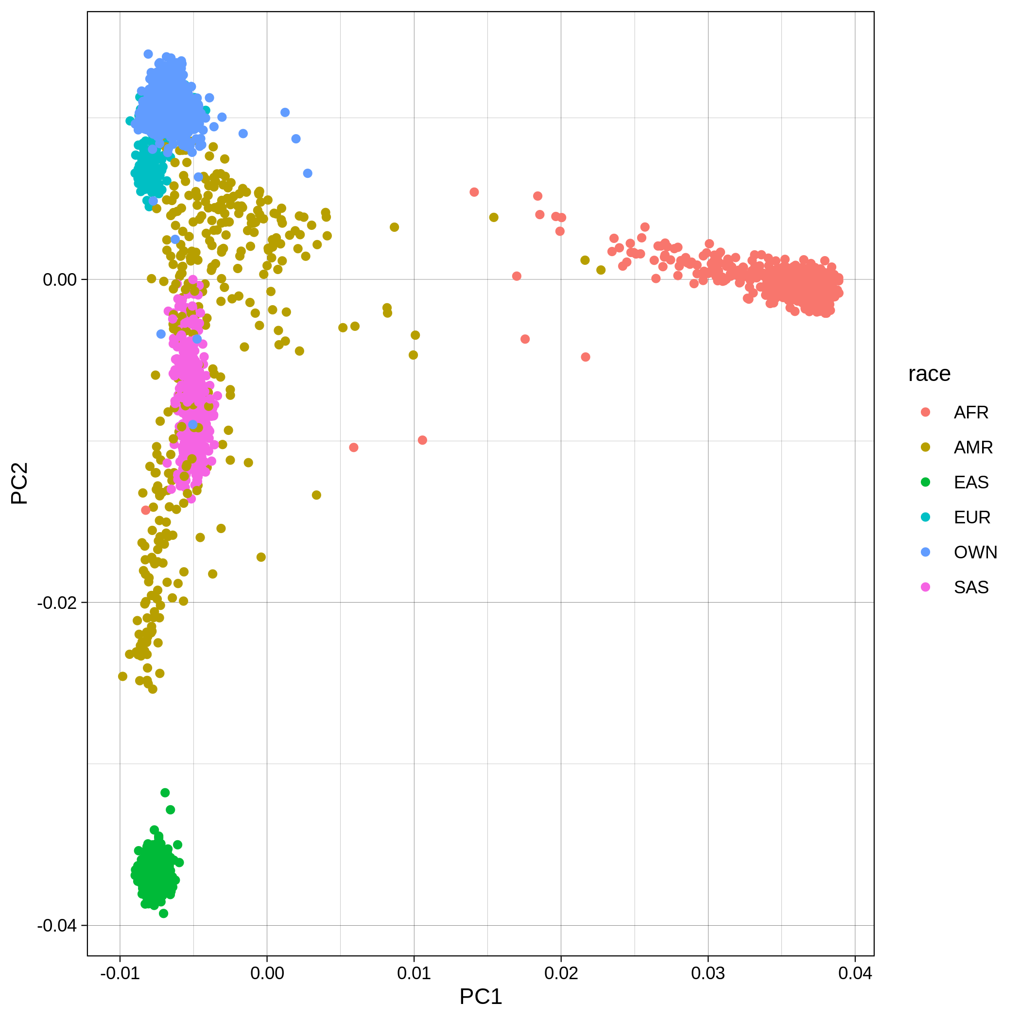 |
| ALS dataset: PC1vsPC3 before removal | ALS dataset: PC1vsPC3 after removal |
|---|---|
 |
 |
| ALS dataset: PC2vsPC3 before removal | ALS dataset: PC2vsPC3 after removal |
|---|---|
 |
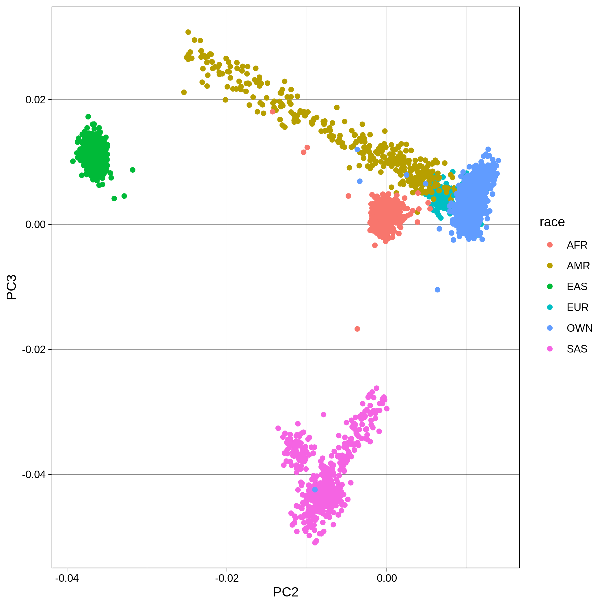 |
| ALS dataset: 3D PCA before removal | ALS dataset: 3D PCA after removal |
|---|---|
 |
 |
You can notice that the ALS dataset still contains some outliers after the automatic outlier removal, this is because we used the default parameters of smartpca. This behaviour can be altered providing an external parfile as explained here. Below we show an example of a more strict outlier removal using the following parfile:
numoutlierevec: 7
outliersigmathresh: 4
To use an external parfile in population stratification, you can run the following command:
nextflow run main.nf -profile standard,conda -params-file parameters.yaml --bed als.bed --bim als.bim --fam als.fam --qc --gwas --pop_strat -resume --results results_als/ --parfile parfile.txt
These are the removed samples and variants for the toy and the ALS datasets through all the steps of the population stratification:
| Toy removed samples log in population stratification | Toy removed variants log in population stratification |
|---|---|
 |
 |
| ALS removed samples log in population stratification | ALS removed variants log in population stratification |
|---|---|
 |
 |
Note
To remember the codes for each step visit the Workflow Descriptions section.
Genome-Wide Association Study --gwas
Within the results_toy/gwas/ folder you will see:
- One HTML report including all the following plots
- Three folders:
logs/,figures/andbfiles/.
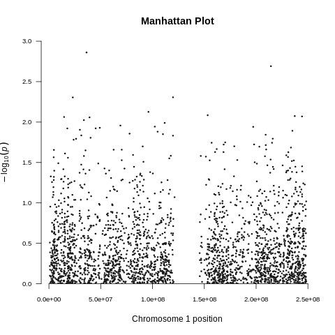
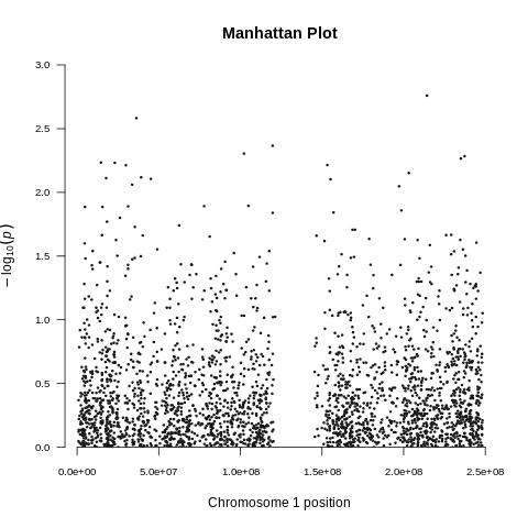
| Toy dataset: Manhattan plot | Toy dataset: Manhattan plot with no covariates |
|---|---|
 |
 |
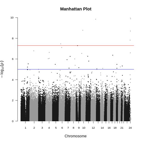
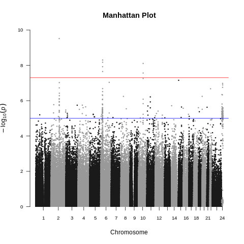
| ALS dataset: Manhattan plot | ALS dataset: Manhattan plot with no covariates |
|---|---|
 |
 |
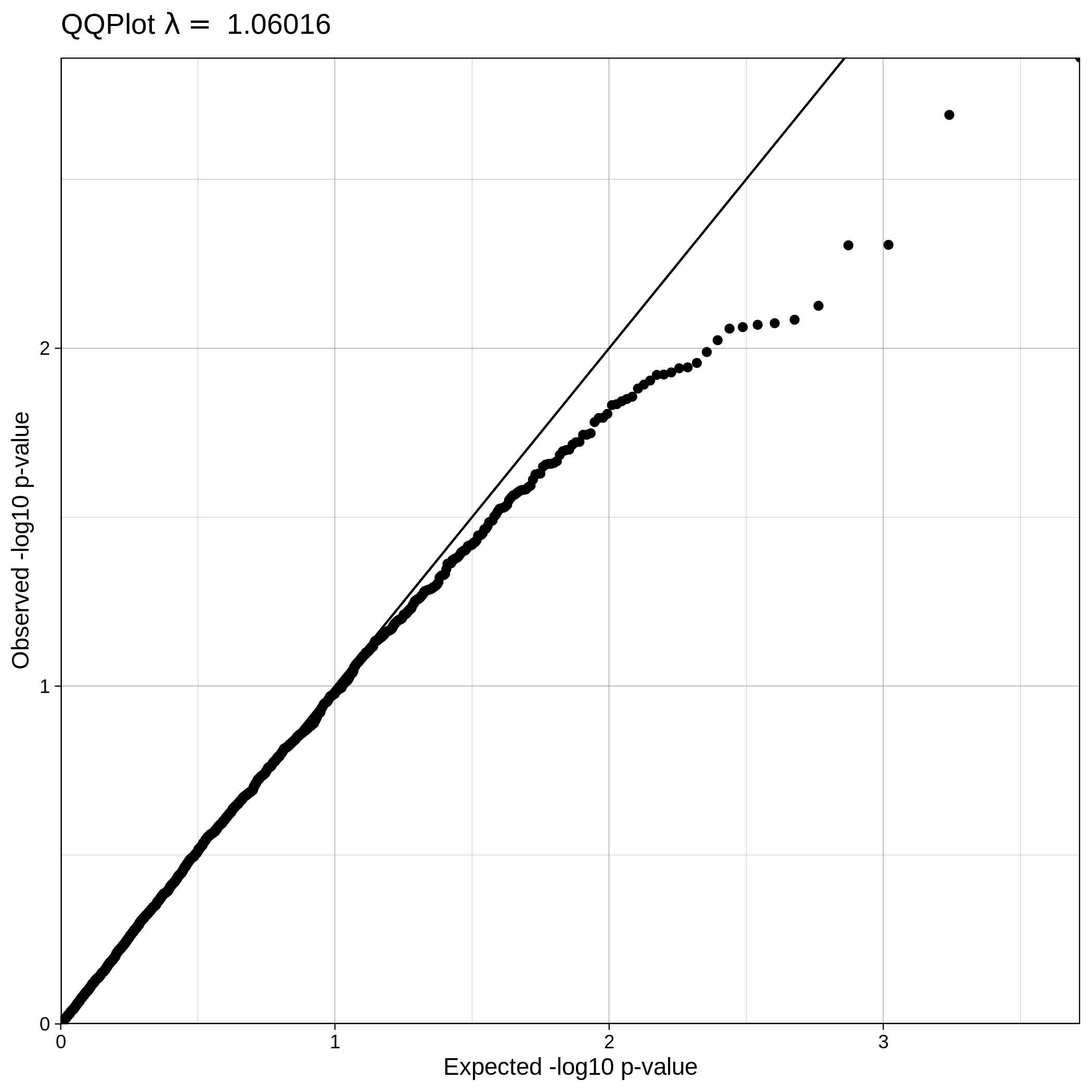
| Toy dataset: Q-Q plot | Toy dataset: Q-Q plot with no covariates |
|---|---|
 |
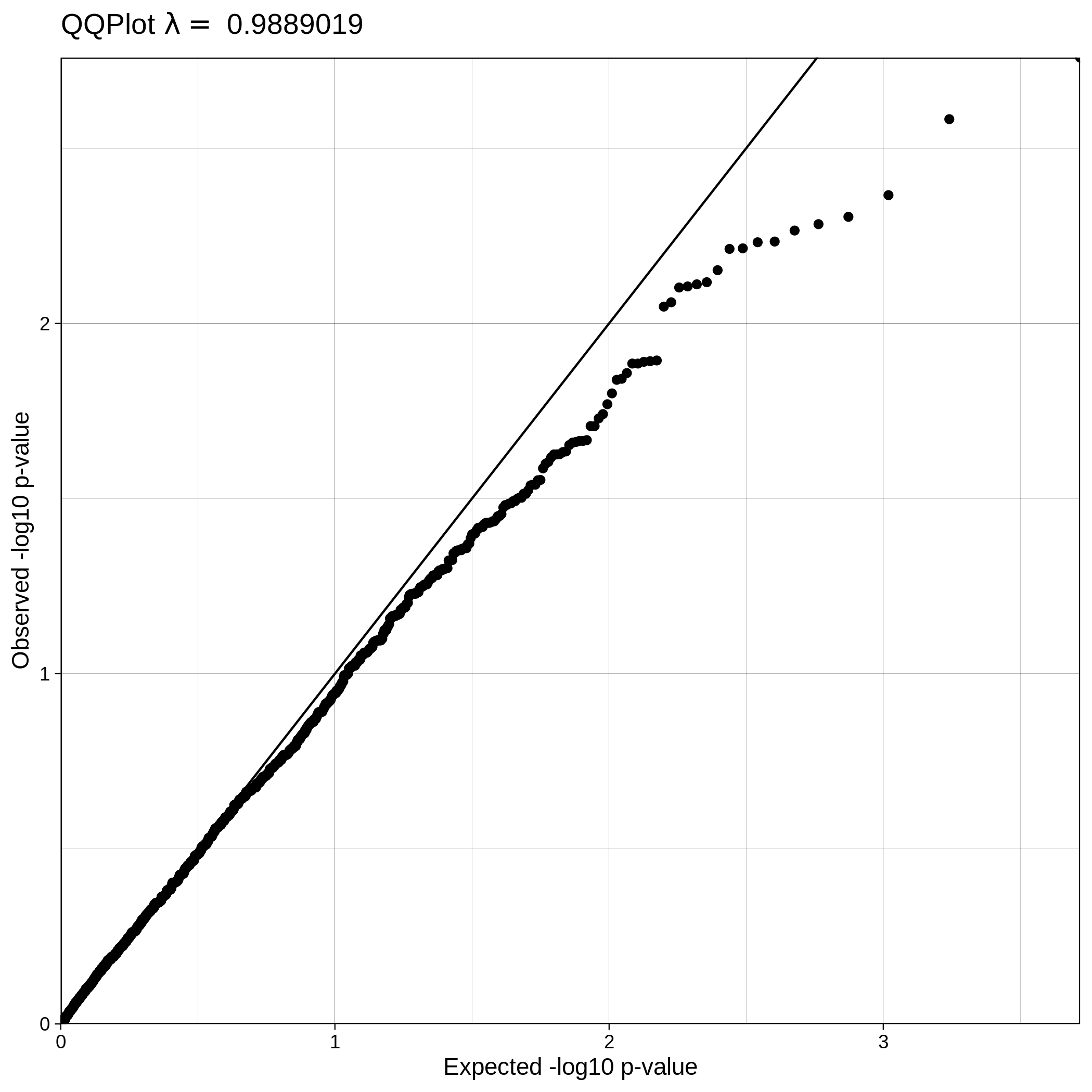 |
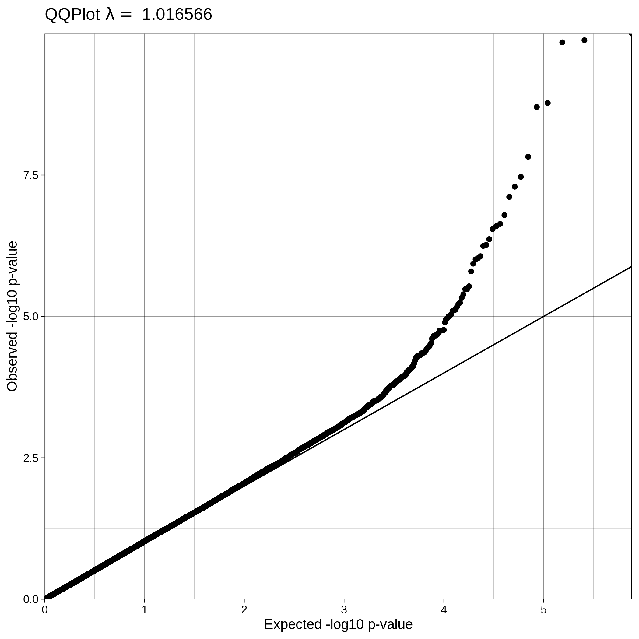
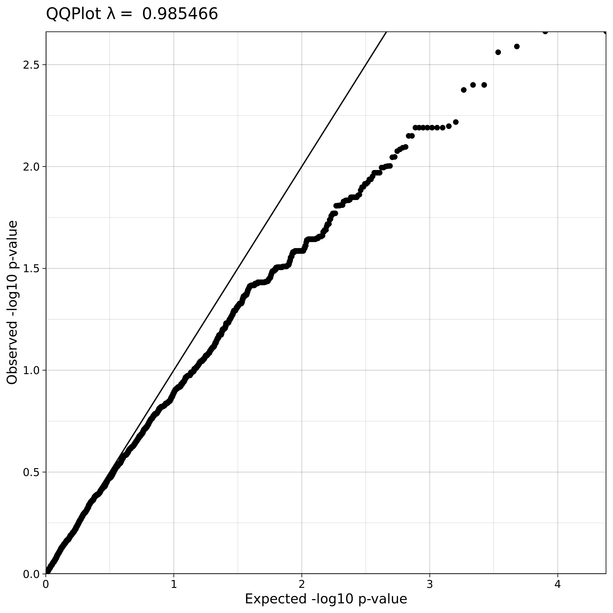
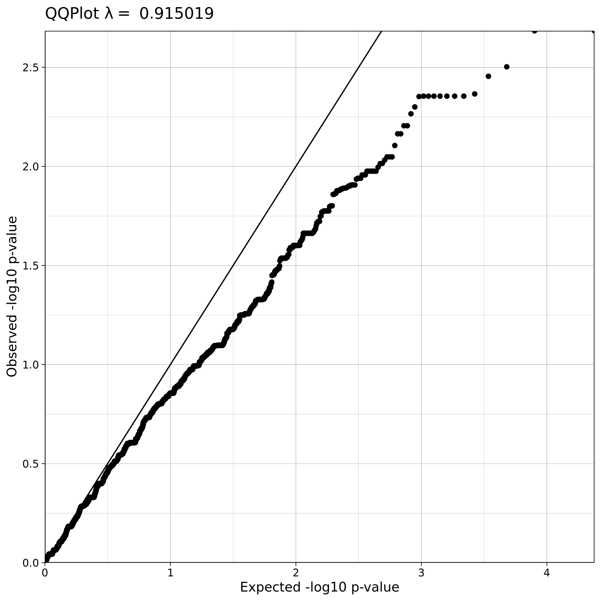
| ALS dataset: Q-Q plot | ALS dataset: Q-Q plot with no covariates |
|---|---|
 |
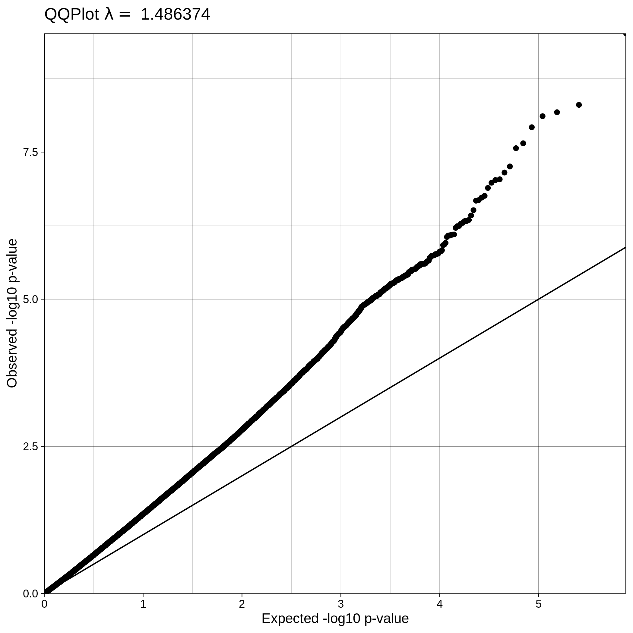 |
Note
The Q-Q plot for ALS data with covariates has a lower lambda value, much closer to 1, which reflects a clean and good quality dataset. This is not the case for the ALS dataset where covariates were not used, which demonstrates that population stratification is an important step, accounting for inner population structure.
Imputation
snpQT offers an optional Imputation workflow where the user can increase the number of markers of their genomic datasets using EBI's phased latest release 1,000 human genome reference panel aligned in human genome build 37.
If you wish to run Imputation locally you should run the following line of code:
nextflow run main.nf -profile standard,singularity -params-file parameters.yaml --bed data/toy.bed --bim data/toy.bim --fam data/toy.fam --qc --pop_strat --gwas --impute -resume --results results_toy_imputed/ --sexcheck false
Tip
- You can use
-profile standard,docker(Docker requires root access so you can use it only on a standard laptop),-profile [standard/cluster],singularityor-profile cluster,modulesto run imputation. - Imputation needs
--qcto run (--pop_stratis optional but it is recommended). - Use
--gwasif you want to acquire genotype-phenotype associations in the imputed data. - If you have already used
--qc,--pop_stratand--gwas, you can use-resumeto savesnpQTfrom spending valuable time by picking up the analysis where you left it, using nextflow's continuous points. - The
--imputeworkflow runs automatically the pre-imputation and post-imputation QC workflows.
Note
The following parameters: --bed data/toy.bed, --bim data/toy.bim, --fam data/toy.fam and --qc could have been omitted from the command above, as they are aready have these values in the parameters file, but we display them here for emphasis.
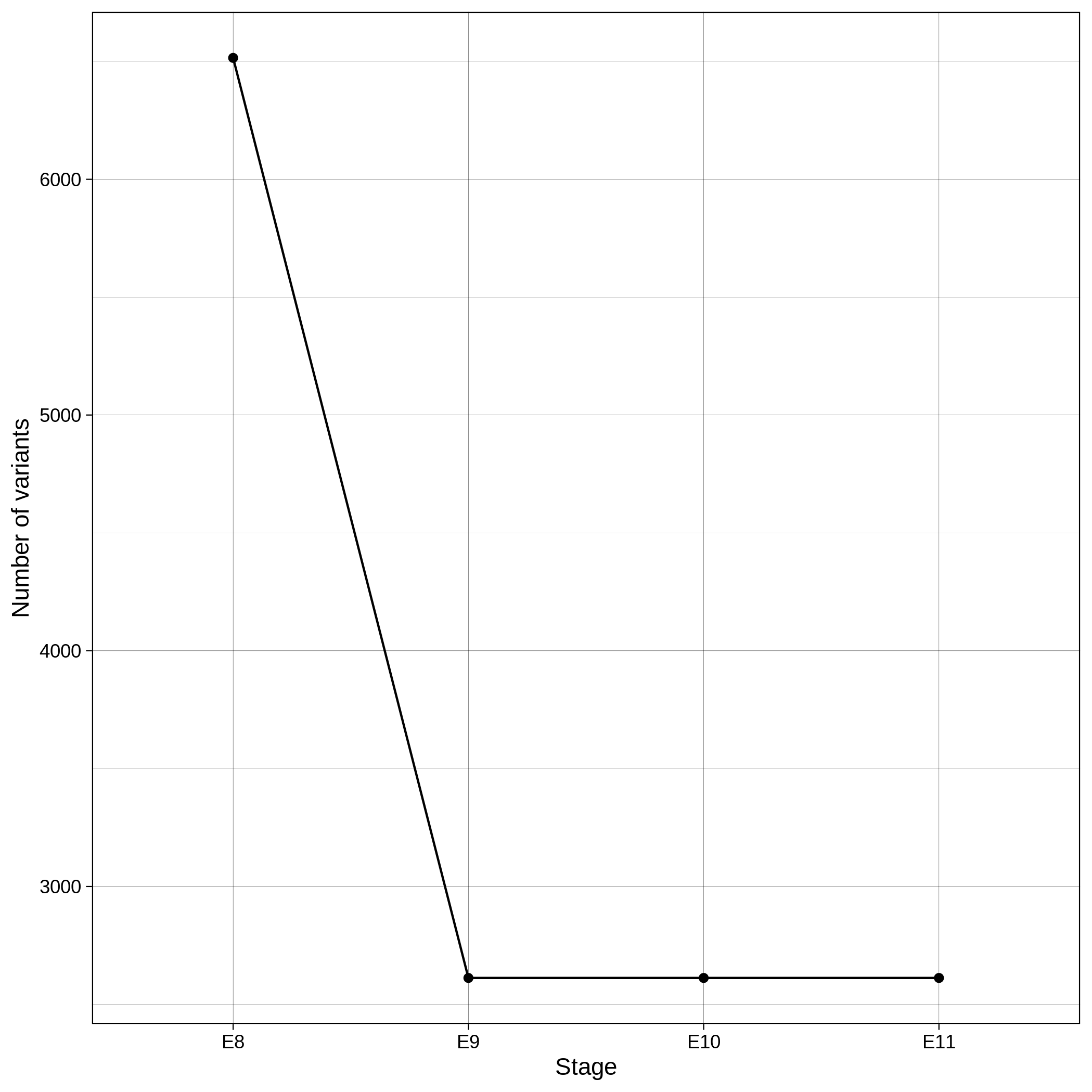
Pre-Imputation, Imputation & Post-Imputation --impute
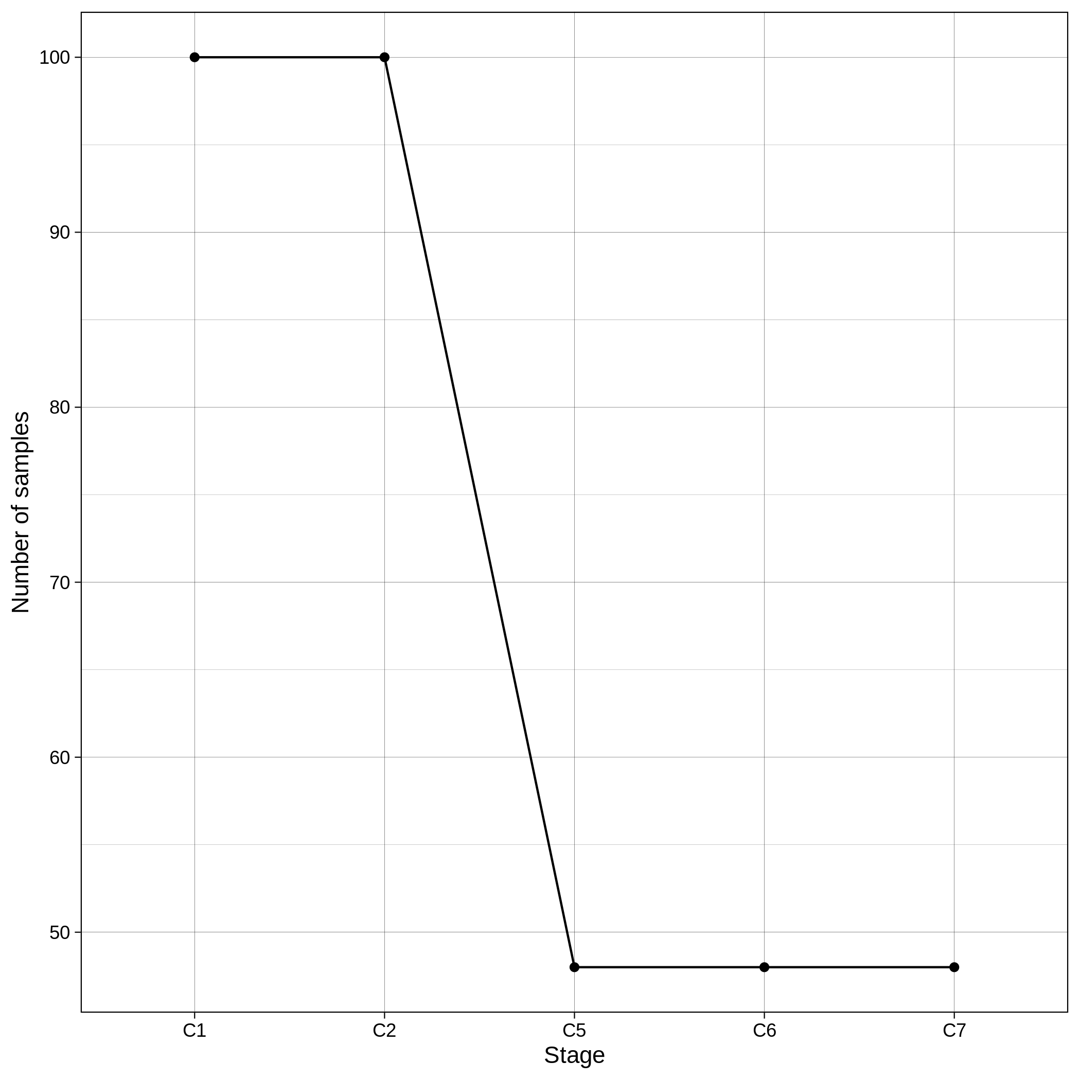
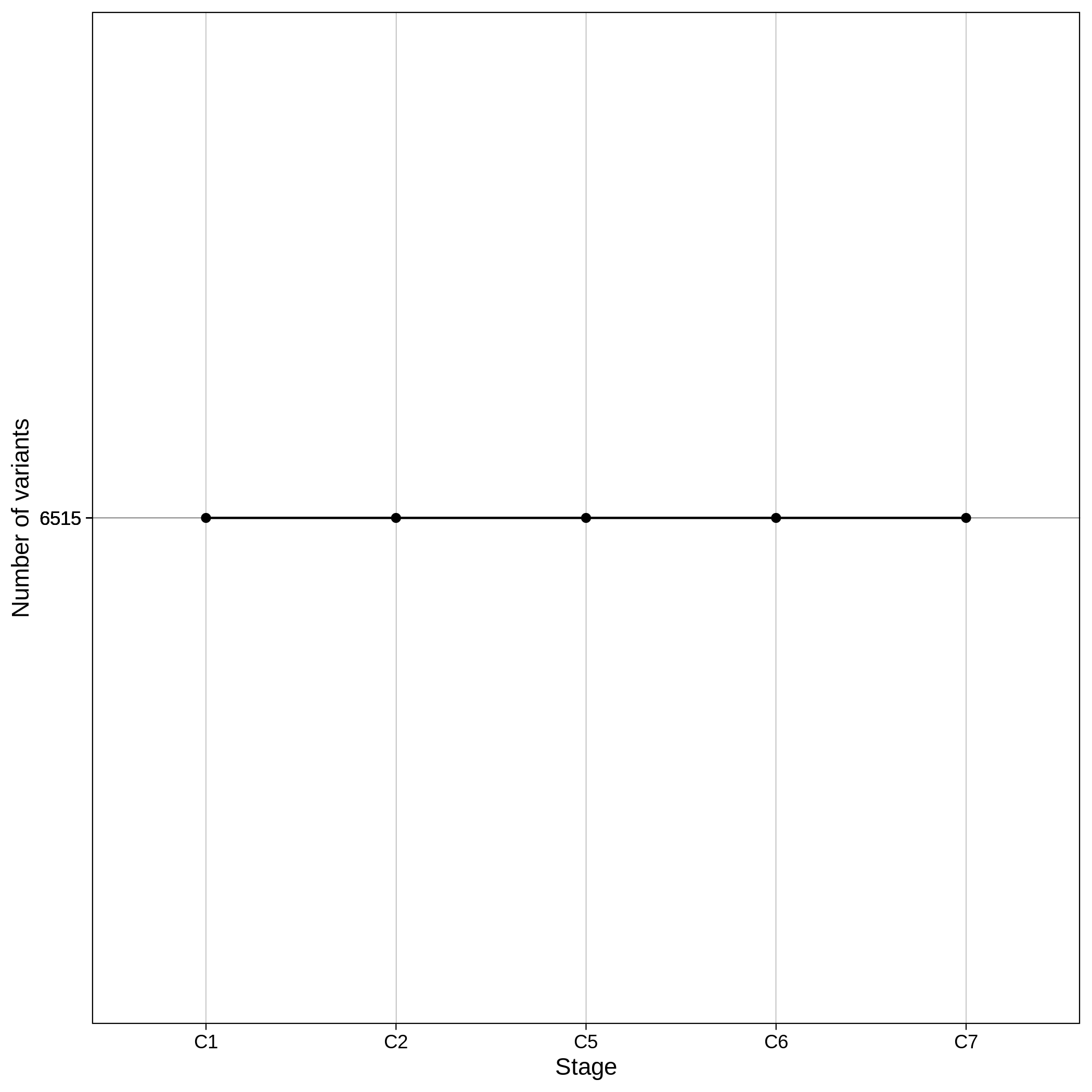
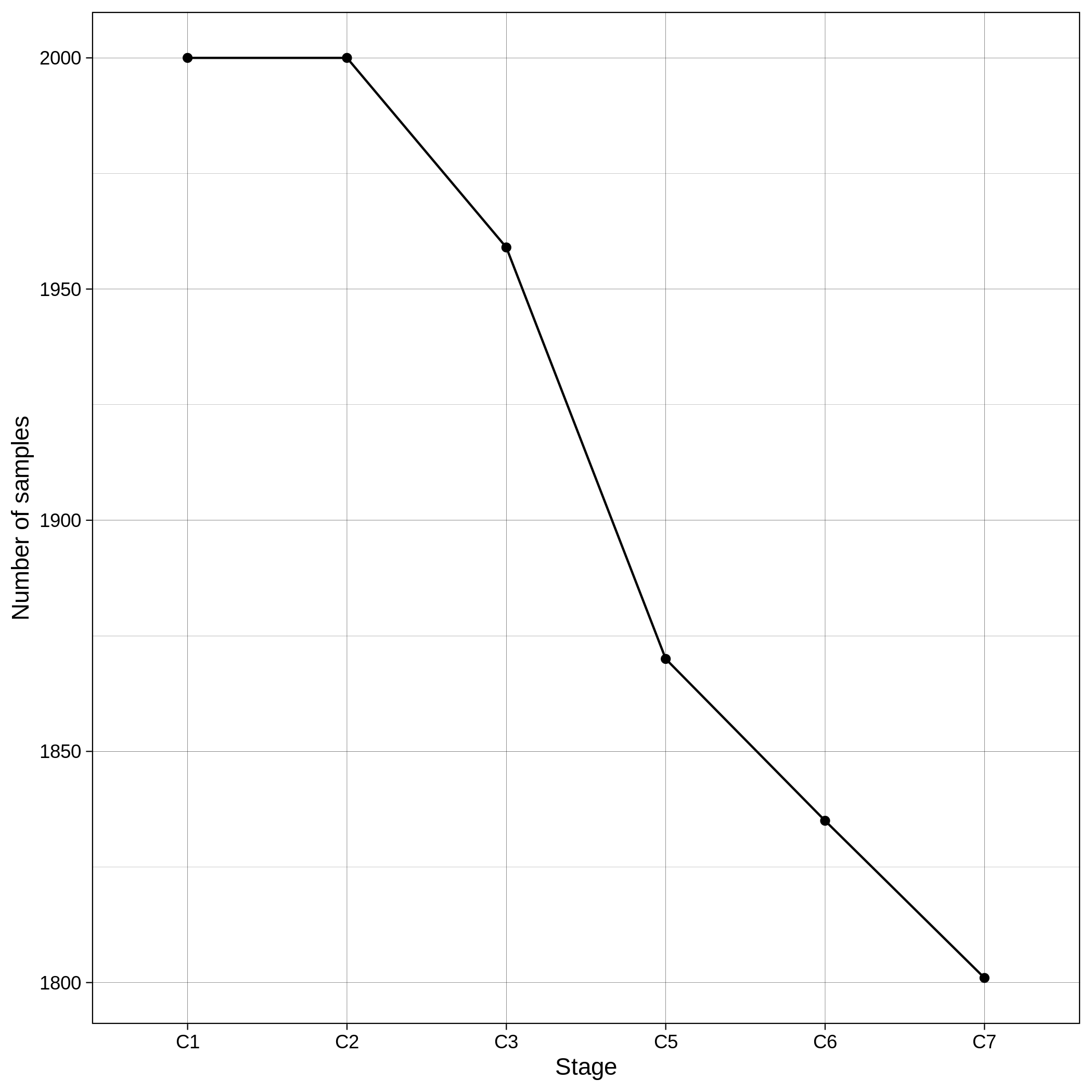
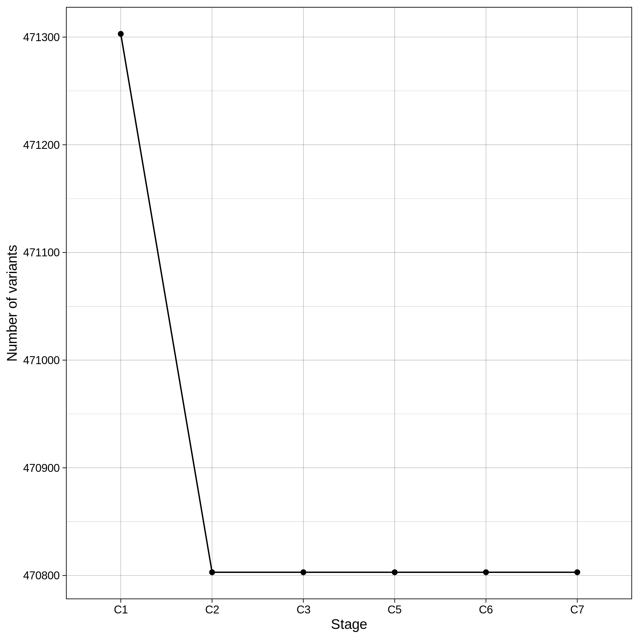
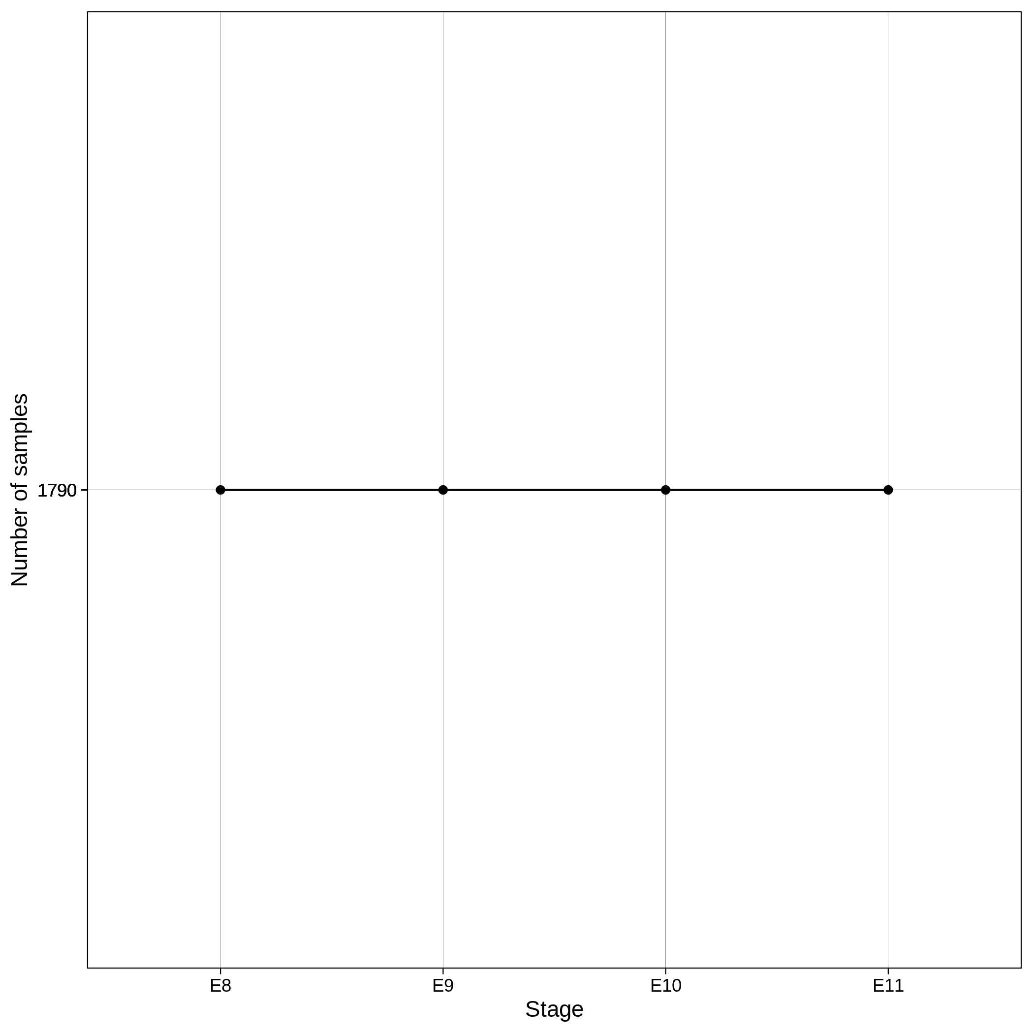
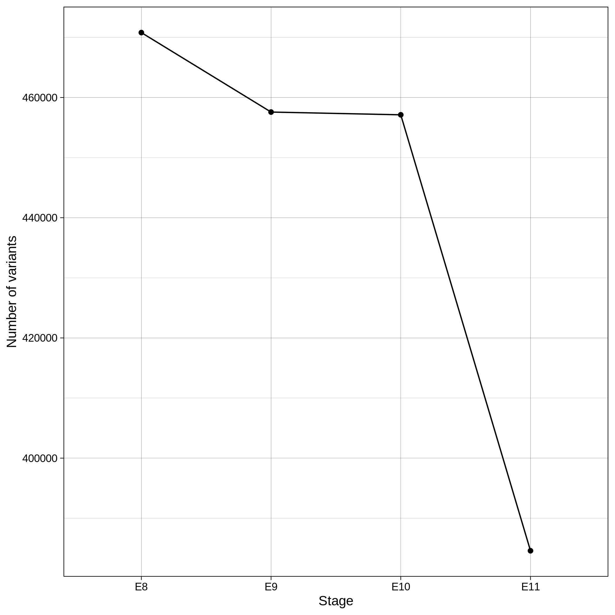
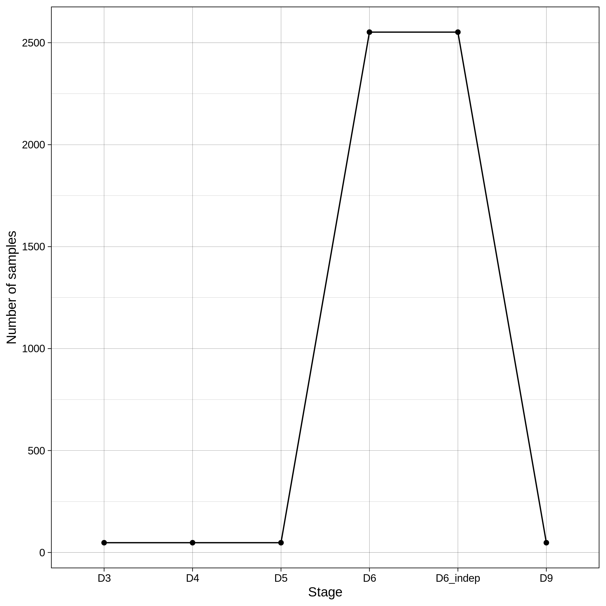
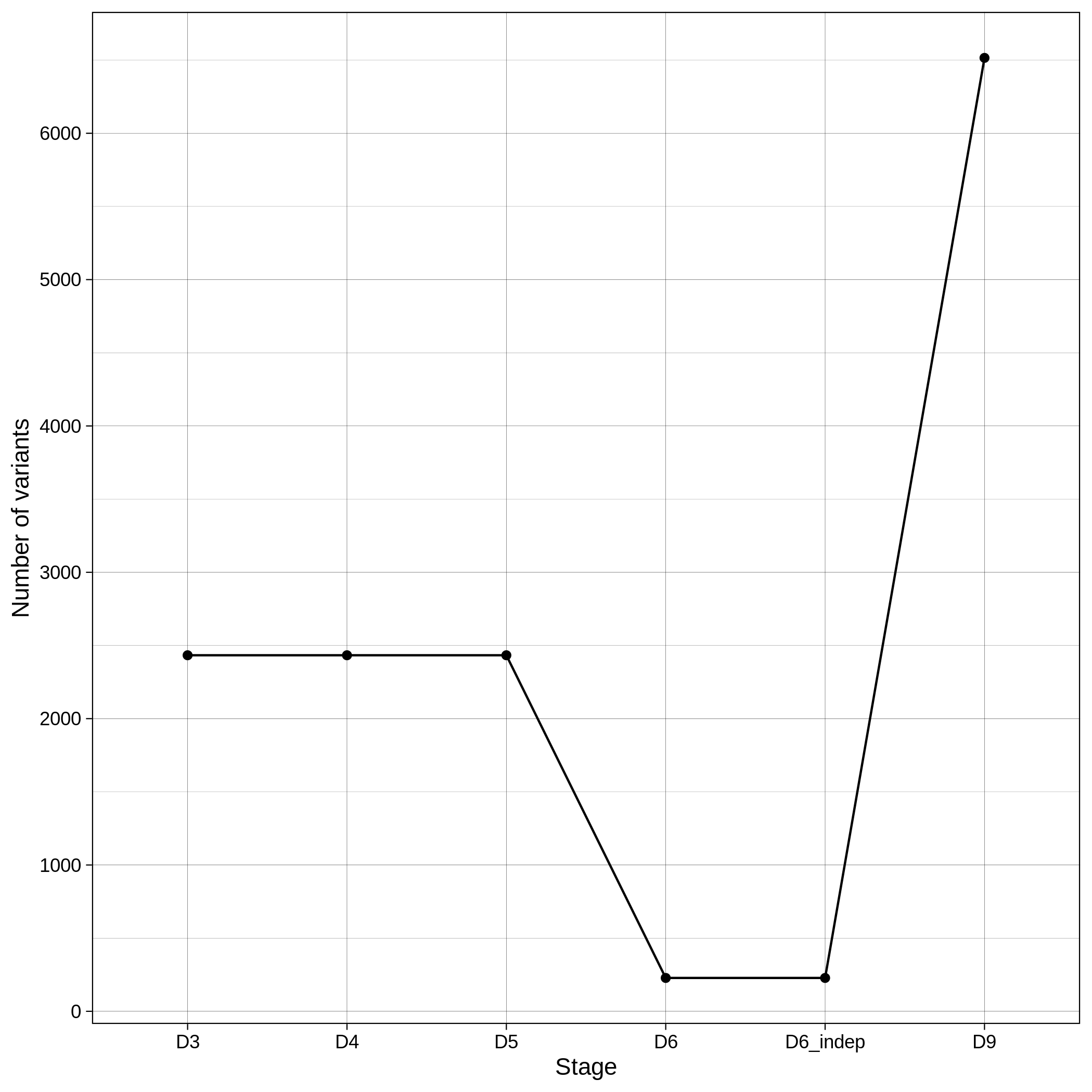
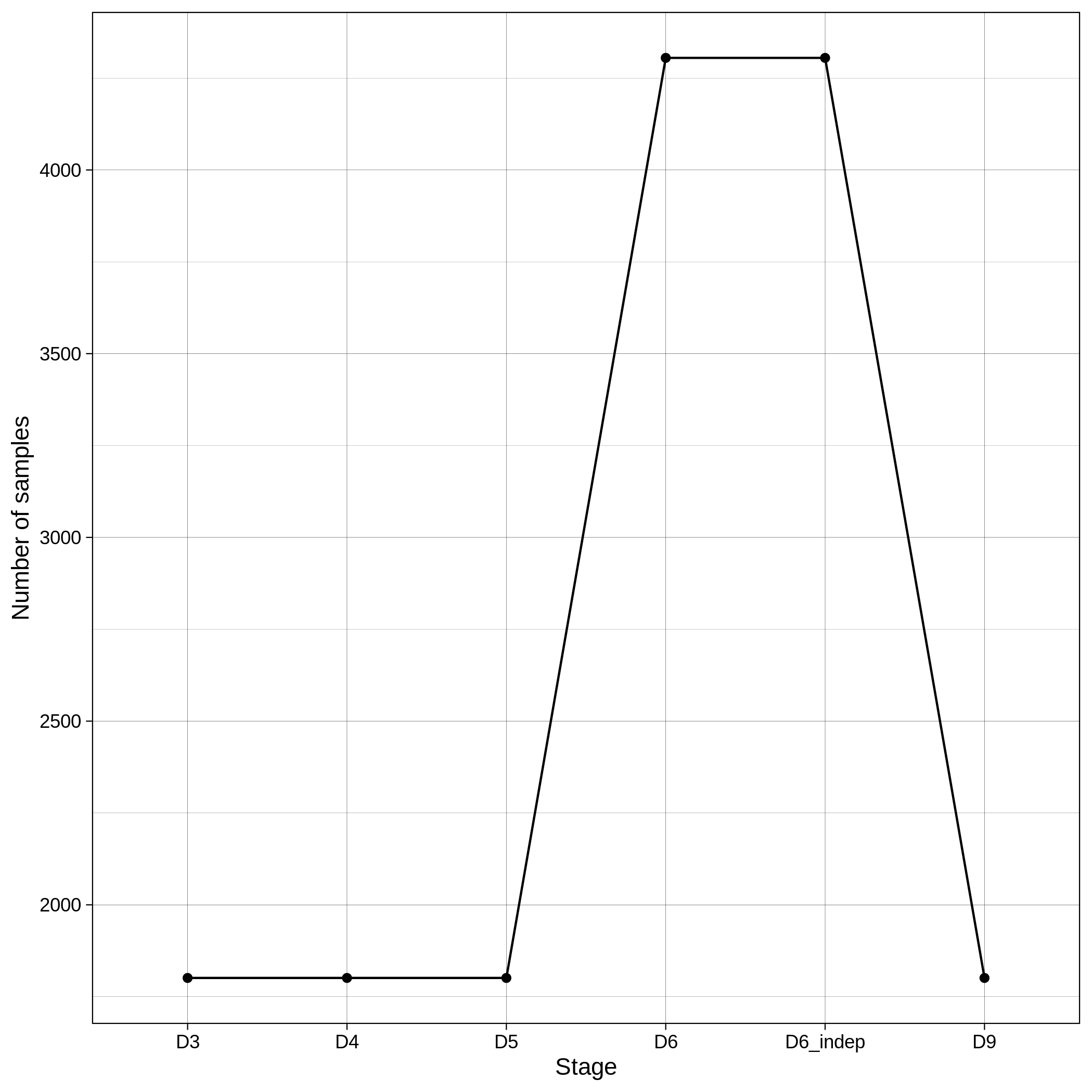
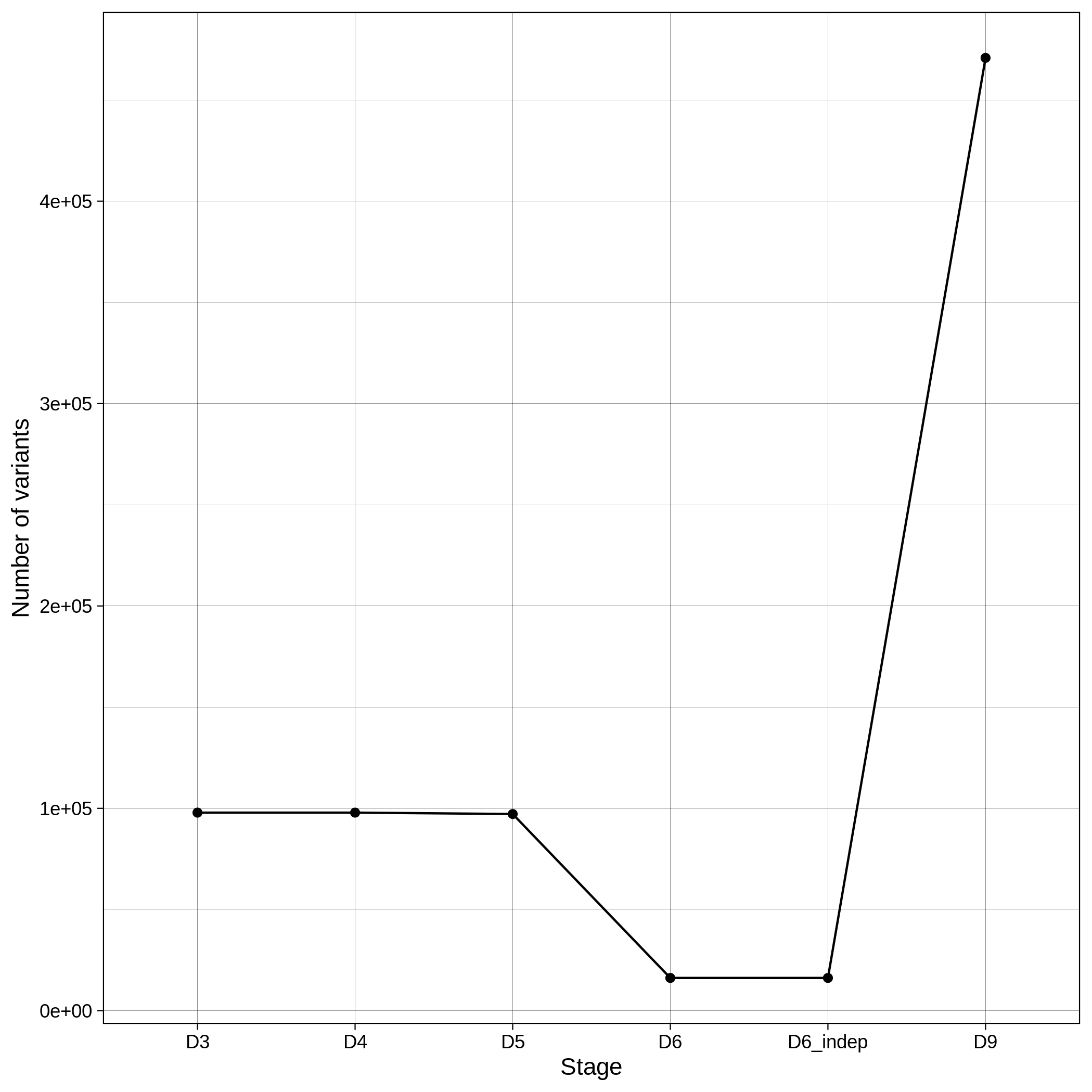
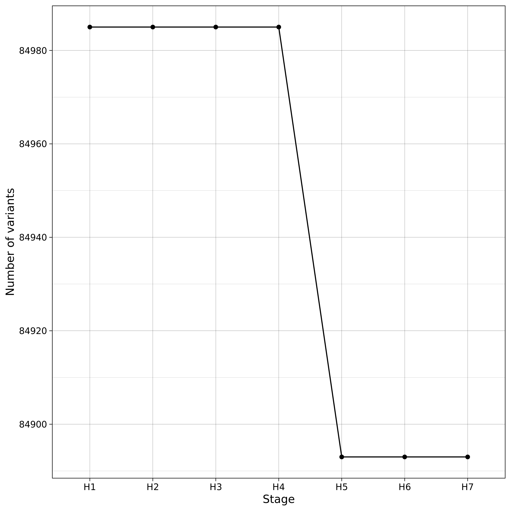
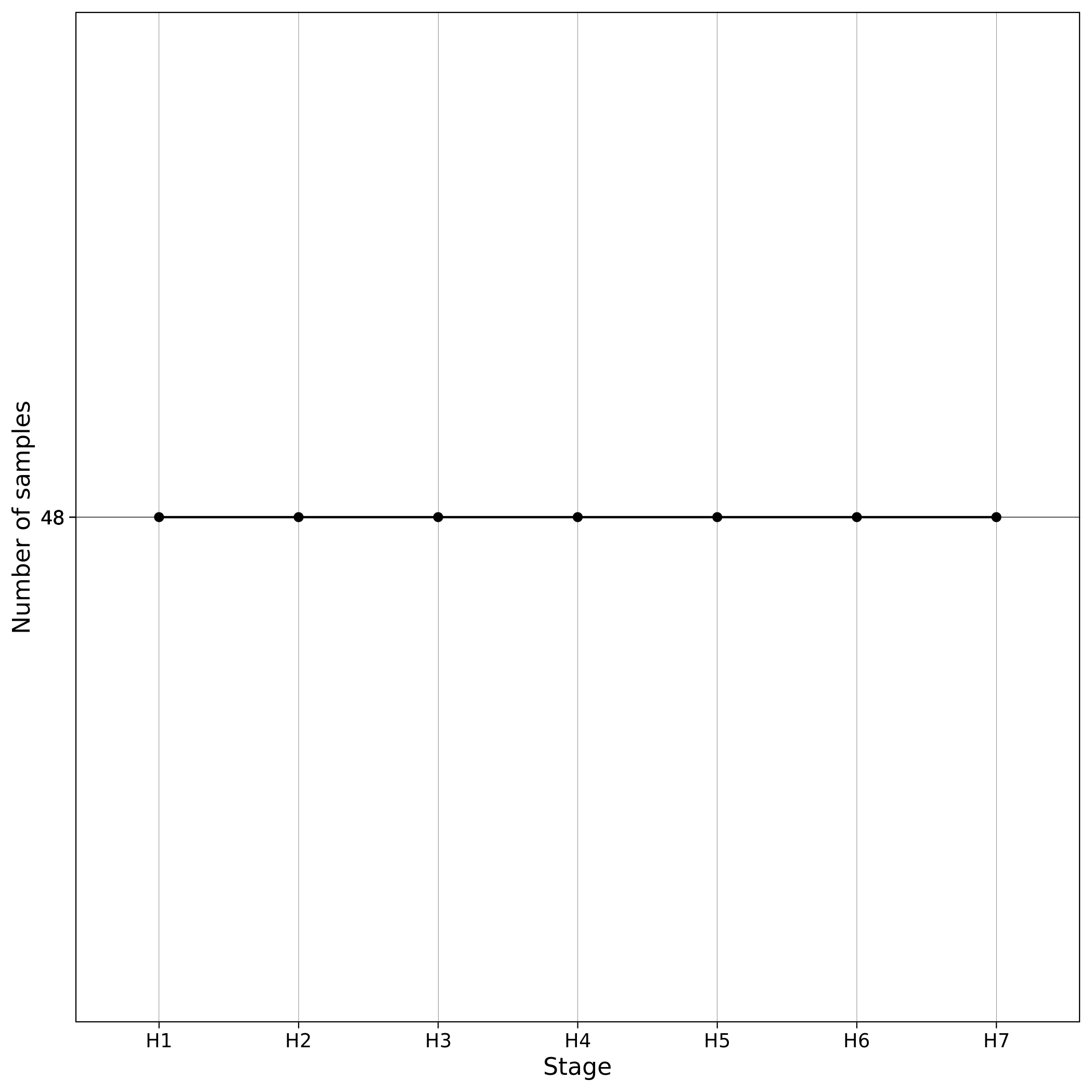
When --impute workflow parameter is used, pre-imputation, local imputation and post-imputation are performed. In our servers, all the imputation- related workflows and GWAS took less than 10 minutes to complete using the toy dataset. When Imputation is finished the toy dataset contains 6,500,533 variants located in chromosome 1. Those variants are then further processed and filtered in the Post-Imputation QC workflow. You can see below log graphs illustrating the number of the remaining variants and samples for each step. All the checks in Post-Imputation are performed in variants, but to ensure again that nothing went wrong we also provide details about the number of samples (which remain the same).
| Toy: Number of variants per step in Post-Imputation | Toy: Number of samples per step in Post-Imputation |
|---|---|
 |
 |
| ALS: Number of variants per step in Post-Imputation | ALS: Number of samples per step in Post-Imputation |
|---|---|
|
|
Note
- You can inspect the exact number of variants and samples per step in the
results_toy/post_imputation/logs/post_impute_log.txt - You can check what is the purpose of each step of the code here.
Since, the latest EBI 1,000 human genome data release (5b) has removed the variant ids, we annotate all the variants in a "chromosome:position:reference_allele:alternative_allele" format.
Tip
You can annotate your imputed variants using tools like SnpSift.
Genome-Wide Association Study --gwas
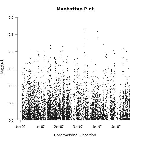
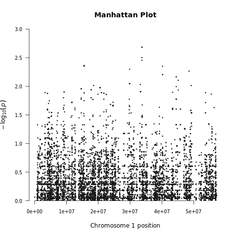
Below we demonstrate the GWAS results of the imputed toy and ALS datasets:
| Toy dataset: Manhattan plot | Toy dataset: Manhattan plot with no covariates |
|---|---|
 |
 |
| ALS dataset: Manhattan plot | ALS dataset: Manhattan plot with no covariates |
|---|---|
|
|
| Toy dataset: Q-Q plot | Toy dataset: Q-Q plot with no covariates |
|---|---|
 |
 |
| ALS dataset: Q-Q plot | ALS dataset: Q-Q plot with no covariates |
|---|---|
|
|
Pre-Imputation
If you wish to perform imputation in an external imputation server or you want to use another reference panel than the latest release of 1,000 human genome data, snpQT is designed to process your data both before and after imputation, with pre-imputation and post-imputation QC workflows, respectively. If you want to clean your dataset and prepare it for imputation, you can run the following line of code:
nextflow run main.nf -profile standard,singularity -params-file parameters.yaml --bed data/toy.bed --bim data/toy.bim --fam data/toy.fam --qc --pop_strat --pre_impute -resume --results results_toy/ --sexcheck false
Note
The following parameters: --bed data/toy.bed, --bim data/toy.bim, --fam data/toy.fam and --qc could have been omitted from the command above, as they are aready have these values in the parameters file, but we display them here for emphasis.
Pre-imputation makes an extra results_toy/preImputation/files/ directory which contains 2,612 variants stored in D11.vcf.gz and an indexed D11.vcf.gz.csi file.
You can check that everything went ok in pre-imputation using the toy dataset, if the output of bcftools +fixref process is the same as the output below. This output is stored in the .command.log file stored in the work directory of the preImputation:check_ref_allele process. You can find this directory when snpQT has finished in the left corner of this process e.g.
[65/3657a7] process > preImputation:check_ref_allele (1) [100%] 1 of 1, ?
In the example above, you can move to work/65/3657a7... (the directory displayed in your machine will probably be different in your case), view the .command.out and check if you have the same output in the toy dataset as the example below:
# SC, guessed strand convention
SC  TOP-compatible  0
SC  BOT-compatible  0
# ST, substitution types
ST  A>C 133 5.1%
ST  A>G 502 19.2%
ST  A>T 0   0.0%
ST  C>A 103 3.9%
ST  C>G 0   0.0%
ST  C>T 553 21.2%
ST  G>A 541 20.7%
ST  G>C 0   0.0%
ST  G>T 118 4.5%
ST  T>A 0   0.0%
ST  T>C 550 21.1%
ST  T>G 112 4.3%
# NS, Number of sites:
NS  total           2612
NS  ref match       1338    51.2%
NS  ref mismatch    1274    48.8%
NS  flipped         0   0.0%
NS  swapped         1274    48.8%
NS  flip+swap       0   0.0%
NS  unresolved      0   0.0%
NS  fixed pos       0   0.0%
NS  skipped         0
NS  non-ACGT        0
NS  non-SNP         0
NS  non-biallelic   0
Warning
--pre_impute workflow can only be used along with --qc and can not be linked to --gwas. You add qc: true and gwas: false in your parameter file or use --qc and --gwas false.
Post-Imputation
--post_impute workflow is designed for users that have imputed data and they wish to perform post-imputation QC. If you wish to perform a post-imputation QC independently on an already imputed VCF file which contains an INFO column, you may run the following line of code:
nextflow run main.nf -profile standard,singularity -params-file parameters.yaml --vcf $WORK_PATH/merged_imputed.vcf.gz --fam results_toy_imputed/qc/bfiles/E11.fam --post_impute --qc false -resume --results results_postImpute_toy/
Tip
- To retrieve the imputed VCF toy file
merged_imputed.vcf.gz, you can navigate to the work/ directory ofimputation:merge_impprocess when running the Imputation workflow (see example above). - You can add
--info 0.7and--impute_maf 0.01parameters to tailor the processing of your imputed data.
Post-imputation makes an extra results_toy/post_imputation/ directory which contains three folders logs/, figures/ and bfiles/.
Warning
- The
--post_imputeparameter can not be linked to any other workflow. For this reason we have added--qc false, to override theqc: trueparameter specified in parameters.yaml. - The
.vcf.gzshould have an INFO column. If not, you should expect to see a PLINK error message that your input dataset does not contain an INFO column. - The
.famfile should contain the exact same samples as the VCF file (E11.fam -the output file of the--qcpipeline would be ideal for this purpose).